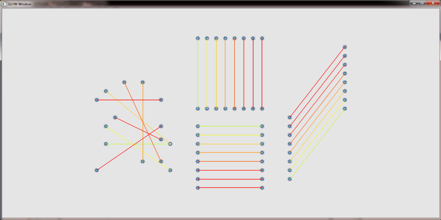
Increase the line size

A further drawback of the pure accumulaton of edges on the GPU is, that we cannot determine the weight of an edge but only the weight of a pixel. Therefore it is not possible to adjust the line width to the weight of an edge. It is however possible to querry neighbouring pixels to determine the weight that colors them. Together with an appropriate distance function that limits the influence of each pixel we can thus reproduce different line widths.

without and with increase line widths:

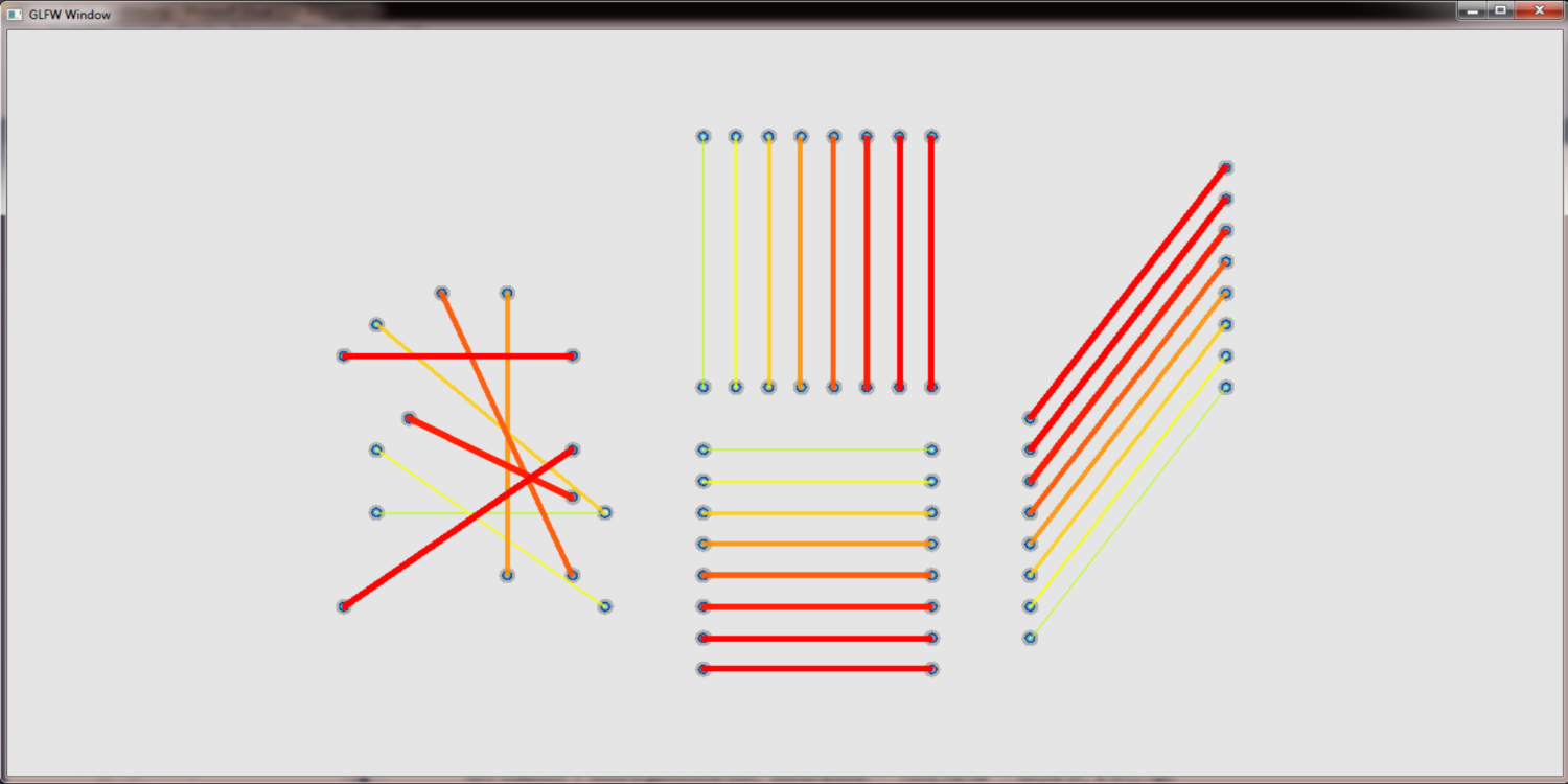
different sample kernels to increase the line width:

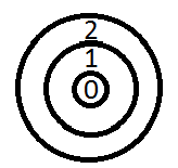
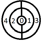
Angle divided rendering to solve crossing problem

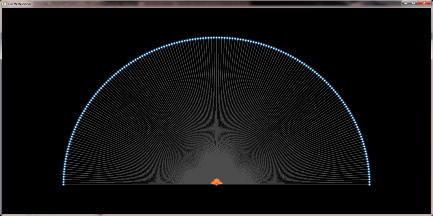
As stated below we have to do the calculations for bundling on the GPU and get the new edge weights on a per pixel basis from additive blending of the edges. One problem that arises from this approach is that edge crossings are counted twice. That missleads the automatic color adjustments and generates artifical heat spots at the crossings. Our solution to this problem is angle divided rendering of edges. Edges with similar angles are less likely to cross and the problem can be reduced beyond visual importance. The more angel sections we use the better the result gets but the process becomes more expensive. Fourtunately with undirected graphs we only have to take care of 180 degrees. Using all 4 color channels (RGB + alpha) we can render 1 degree precision in 45 render passes in realtime on modern GPUs.

rendering in one pass, 180 sectors at a glance and rendering in 45 passes into 4 color channels:

Density field as guidance for edge bundling

QuadTree assisted edge bundling is not sufficient (see results). To improve our results we use the density field to guide edge bundling. The basic idea is a Hill Climbing approach, that moves each edge start / end point from its actual position along the density field to the local center of the gaussian cluster of the edge. This method reduces the set of edges to a set of bundled inter gauss cluster edges, that is way more usefull.
Their are two drawbacks with this new method. First for performance reasons we have to do it on the GPU and therefore loose track of the edges. We can render them at the calculated position but we cannot determine which or how many edges have been merged (we can however use additive blending to get a edge cross count for each pixel). Second on higher zoom levels we get problems with edges that leave the view area and therefore leave the known density field. However the fast and effective bundling of many many edges outweights those problems.
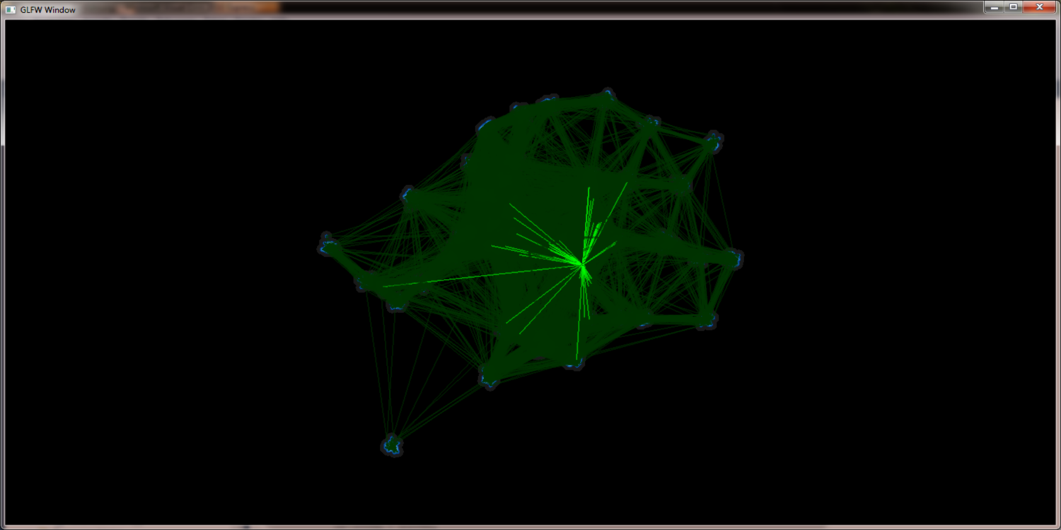
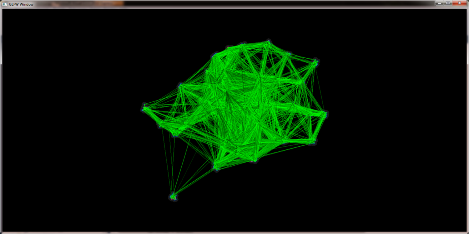
Instead of carrying out the hill climbing calculations for each edge endpoint we calculate it in picture space and get a movement field, that stores for each pixel the position to which edge endpoints are moved. The picture space method makes us independent from the amount of edges.

movement field (pixel color encodes new positions):

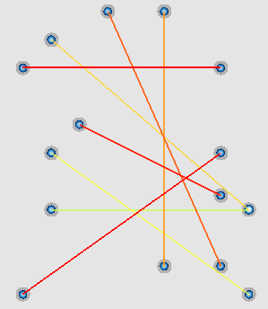
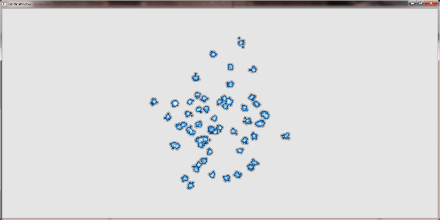
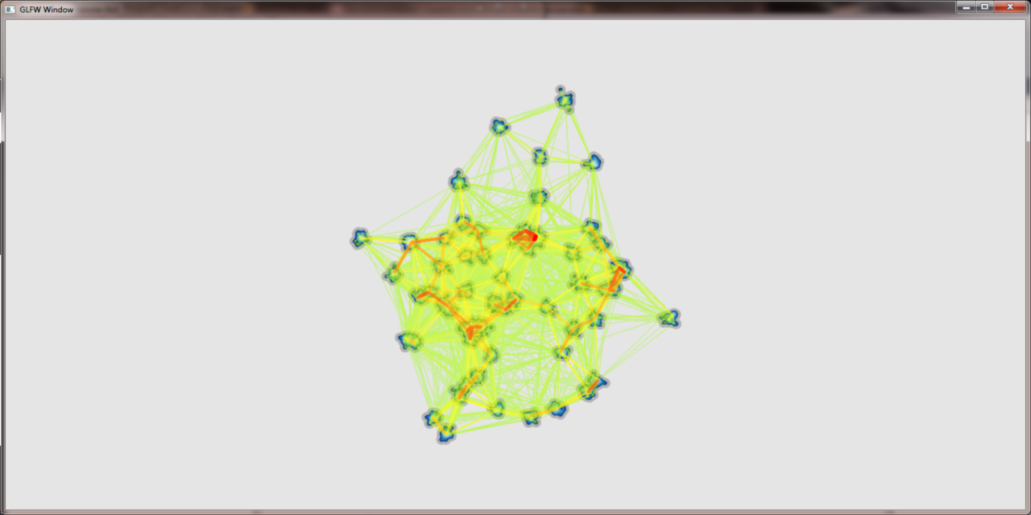
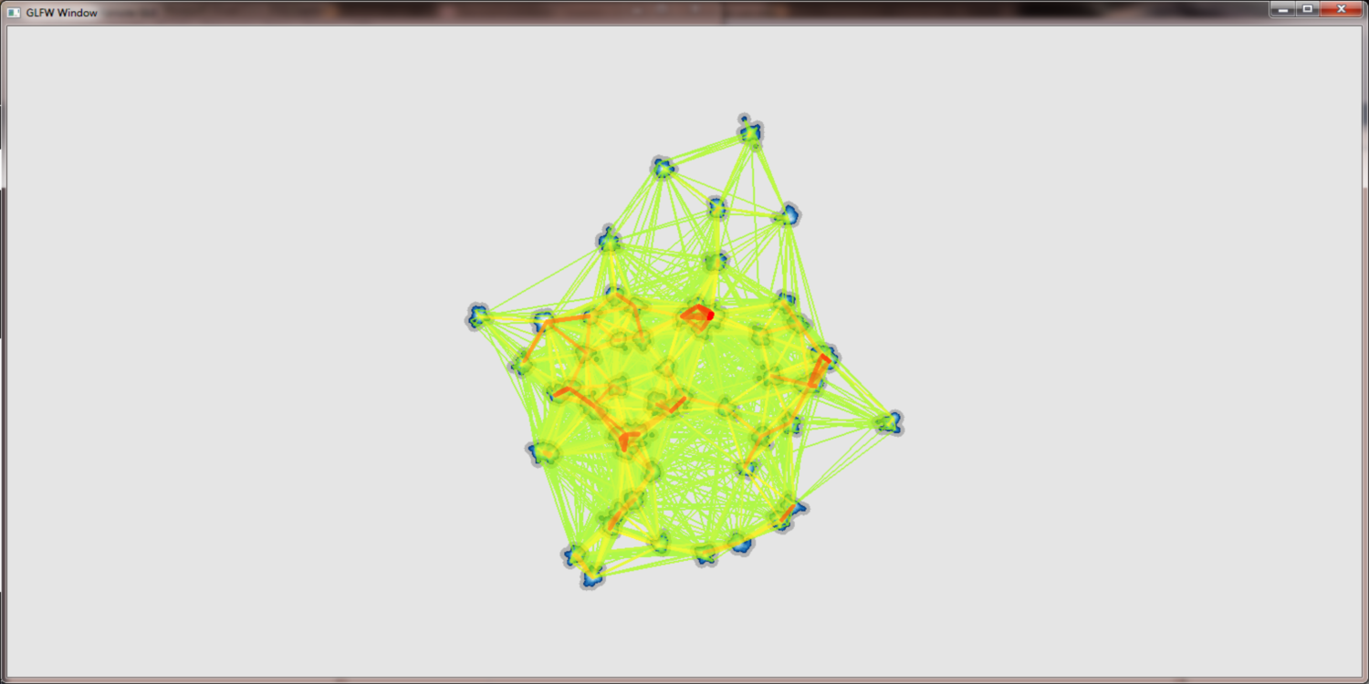
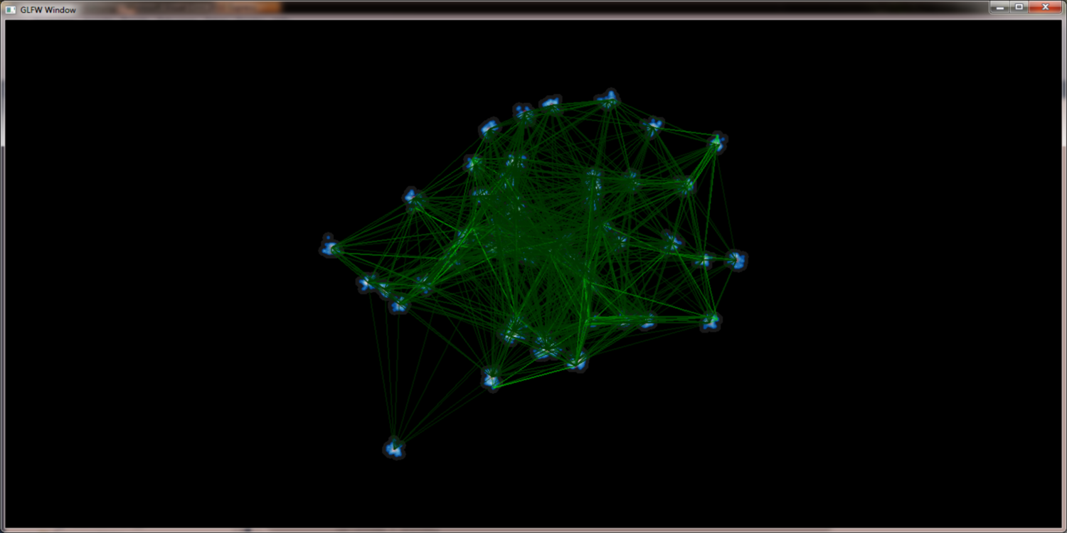
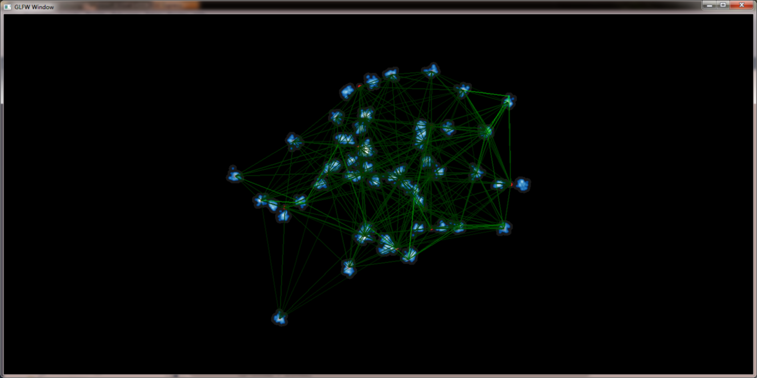
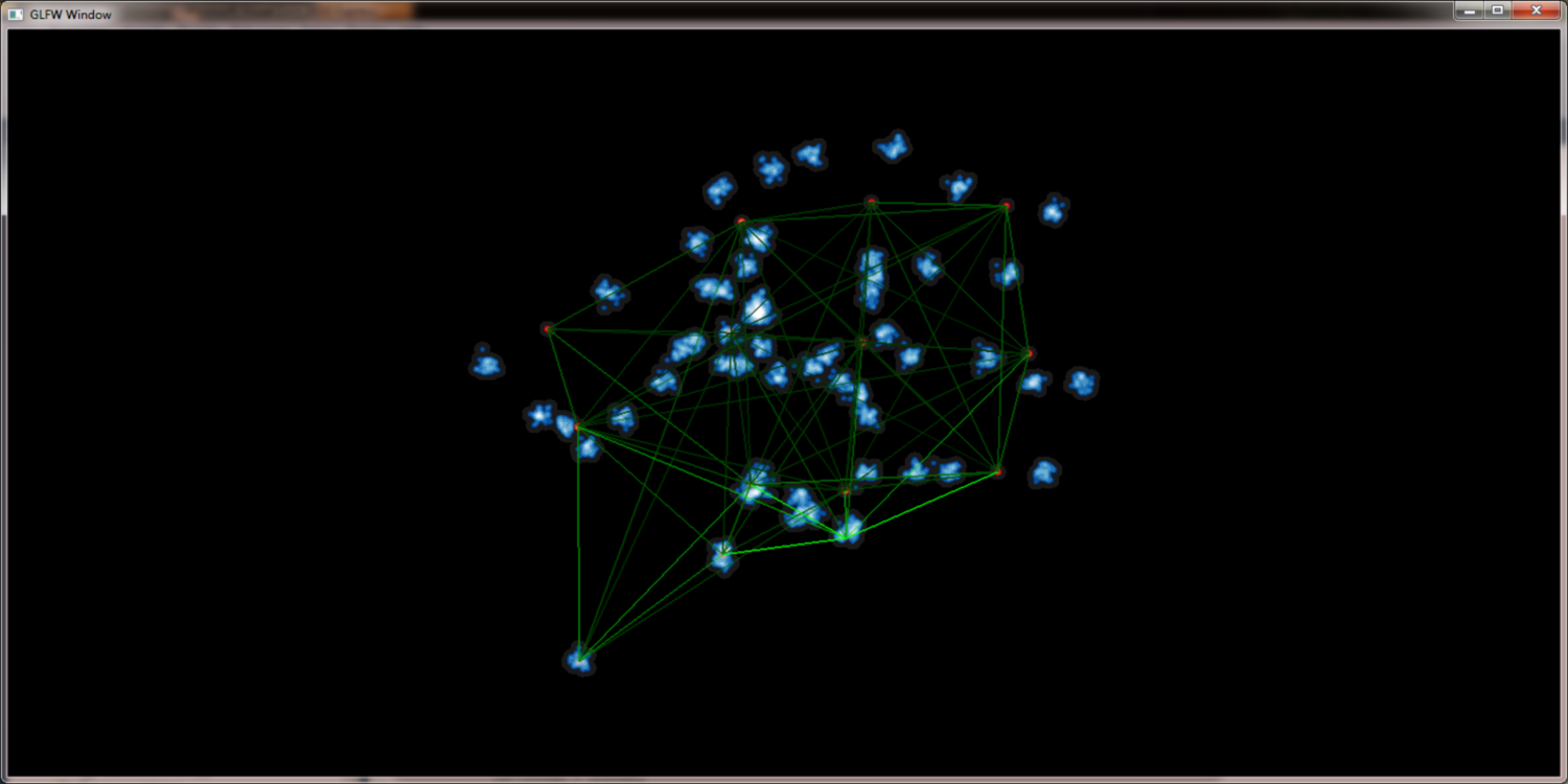
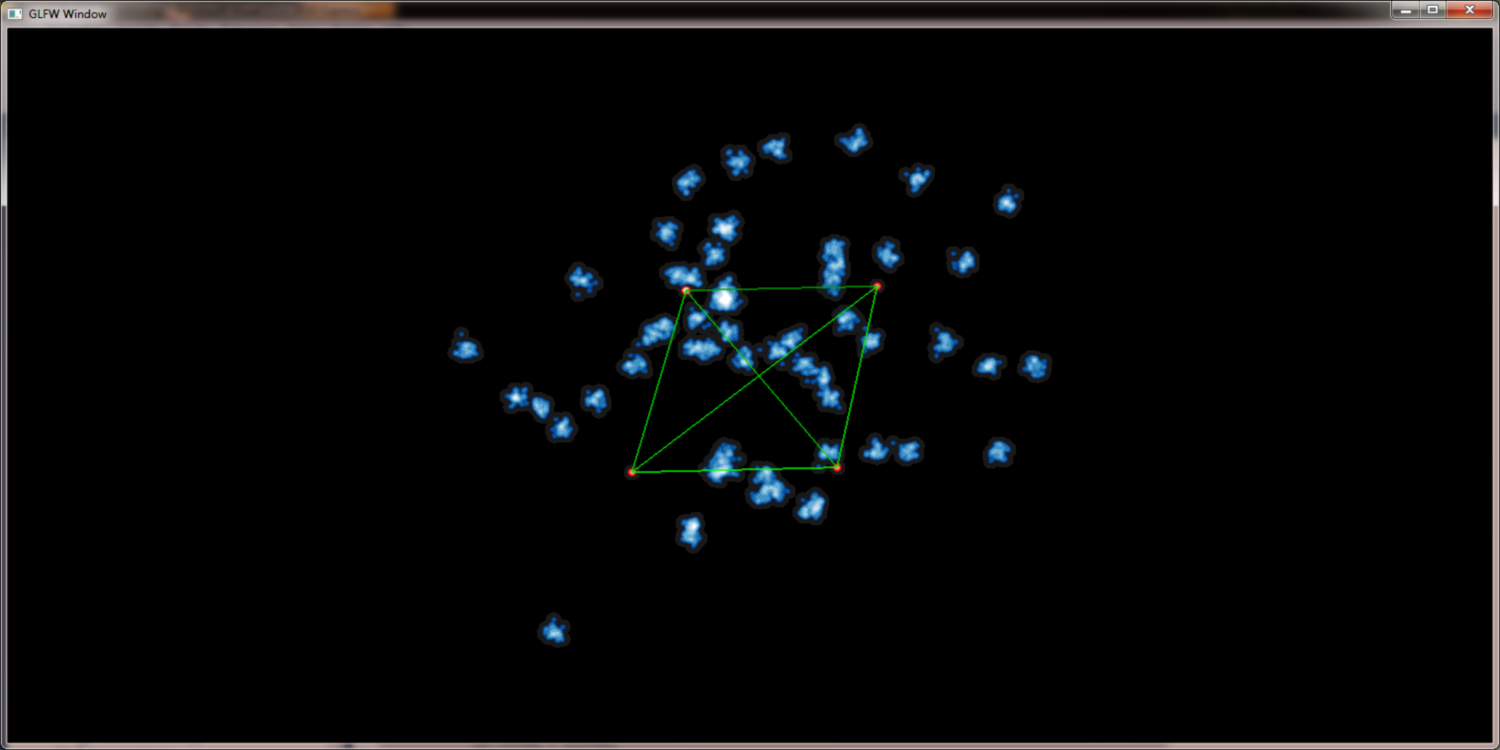
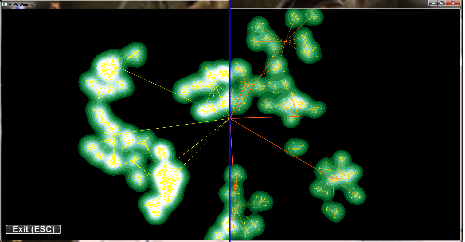
green lines indicate the shift of the edge positions towards the local gaussian clusters:

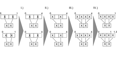
QuadTrees for speed up

To deal with big data sets it is necessary to reduce the amount of gauss kernels the GPU has to deal with. One way to achiev this is to merge points into supernodes. A method that works best if we determine those points that fall into the same pixel anyway. Obviously this reduces the workload of the GPU but at the same time preserves the picture quality. To support the necessary neighberhood querries QuadTrees are well suited because their height is normally near O(log n).

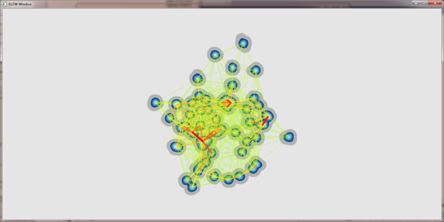
contract nearby nodes to supernodes to increase render speed:

maximal texture value search

To be able to normalize the results obtained throug blending one needs to know the maximal value that results from blending the current picture. Using simple distributed point sets this value can be estimated and set as constant value. For more difficult point sets however this estimation becomes complicated and with varying sigmas a pleasant result can no longer be achieved. Thus we need a method to compute maxima of textures with high performance. Using the CPU to calculate these values has the drawback of increased memory bandwith usage (transfer to main memory) and fast decrasing performance as the pictures become larger. GPUs on the other hand are best used to solve the same small problem lots of times in parallel (in our case get the maximum of a small fraction of the texture). But as the number of problems to solve decreases this advantage dimishs. Clearly the best performance can be achieved by combining both approaches.

The picture shows the generation schema for the max values (see downloads/report)

texture blending

One possibility to apply gaussian kernels on distributed points is to draw them as textures arround the points and then to blend them together to get the accumulated values. The following examples show the process for one and for four (changing) points.

1: send the points to the graphics hardware:

2: use a geometry shader to build rectangles:

3: apply a gaussian texture encoded in the blue value and blend the rectangles into a floating point buffer.

4: use a fragment shader to convert the values to rgb 255:

project DensityPoints - Supersampling

Adding suppersampling helps to deal with aliasing effects on point and edge renderings. On the point rendering (gauss kernel colorings) the image quality improves significant. Improving skew edges is more difficult but while the aliasing artefacts remain in the picture their is still an important improvement in the complete rendering because supersampling increases the visiblity of middrange edges over small edges.

Again the same data set this time with supersampling 4x:

project DensityPoints - HSB coloring and line width

We changed from the hand fitted color map to a HSB based continious representation for the edge colors to increase the information contained in the resulting pictures and to make them more stabel. Furthermore we found a way to increase the width of important lines to draw user attention to important edges. Last but not least accumulated edge values can be scaled similar to nodes, to avoid overdomination of few superstrong connections.

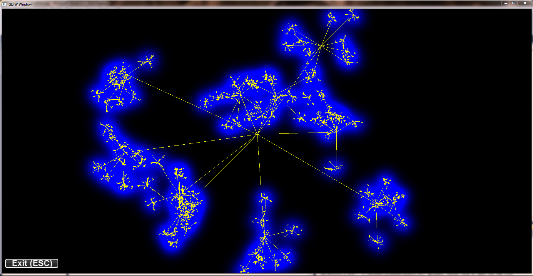
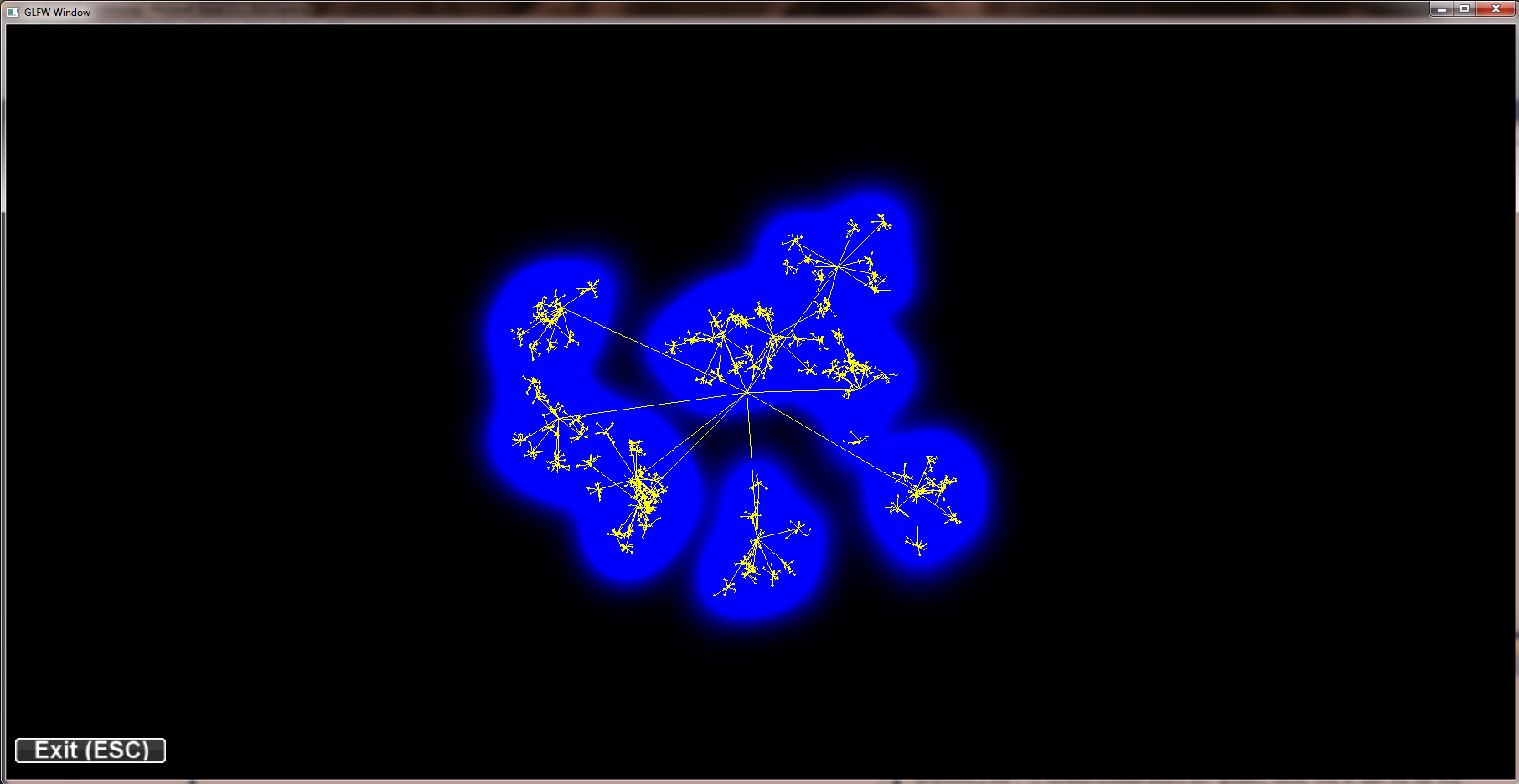
The same data set as below with ^0.25 and ^0.5 scaling and HSB based coloring + line widths:

project DensityPoints - Adding edges 2nd try

With the density field based approach we can achiev much more intuitve edge bundling. Moreover the bundling factor can be easily controlled by the user by adjusting the gaussian kernels. Below we see a artificial hierarchy data set which was rendered with the new approach. While the bundling itself is much better there still remain problems with edge crossings, edge width and the coloring. We used a discret color map that was hand fitted to these data sets for the pictures below.

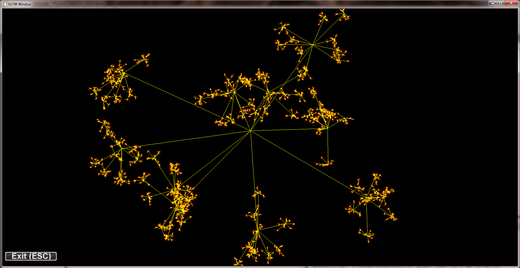
Hand fitted discret color map and density field based edge bundling:

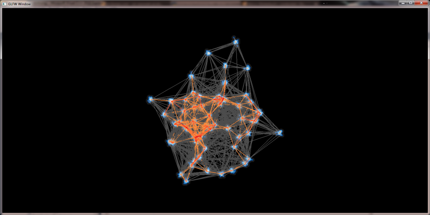
project DensityPoints - Adding edges

Simply rendering the edges into the scene would lead to massive clutter and disturbe the picture. To get a picture that can be read and interpreted by humans some kind of edge highlighting or edge bundling has to be applied. One obvious method to achiev this is to use the (Node)QuadTree to merge the edges. With a set of edges E = { e1{n1,n2}, e2{n3,n4}, ...} where n1 and n3 merge to n13 and n2 and n4 merge to n24 the edges e1 and e2 would merge into e12. While this approach seems promissing the results are not as good as expected. There are too less distinct bundling levels and selecting the correct level remains as problem. Furthermore selecting node merging and edge bundling from different tree levels leads to confusing results.

The edge hierarchy for a given graph using alpha blending to increase edge contrast:

project DensityPoints - Tackling larger data sets

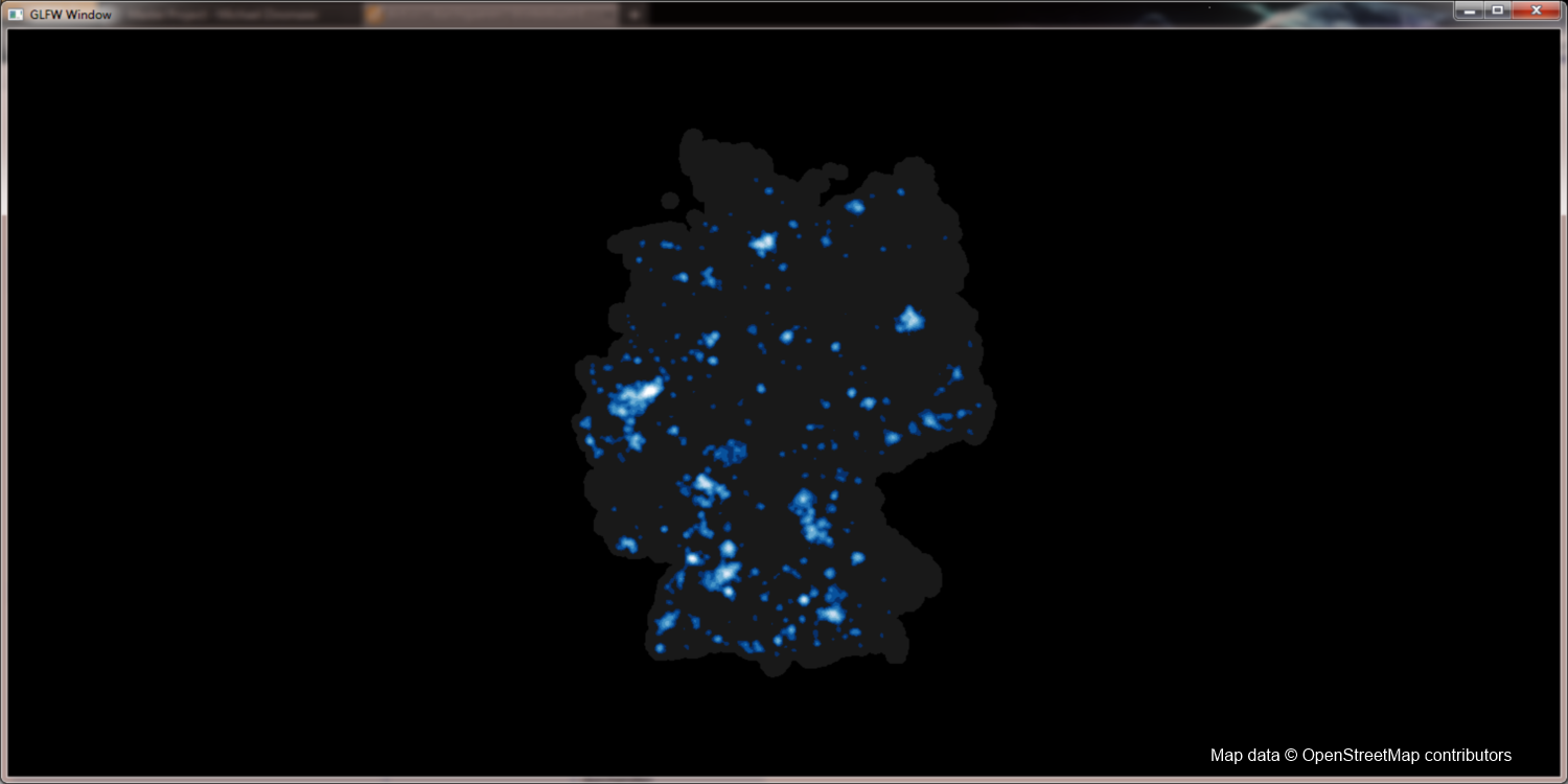
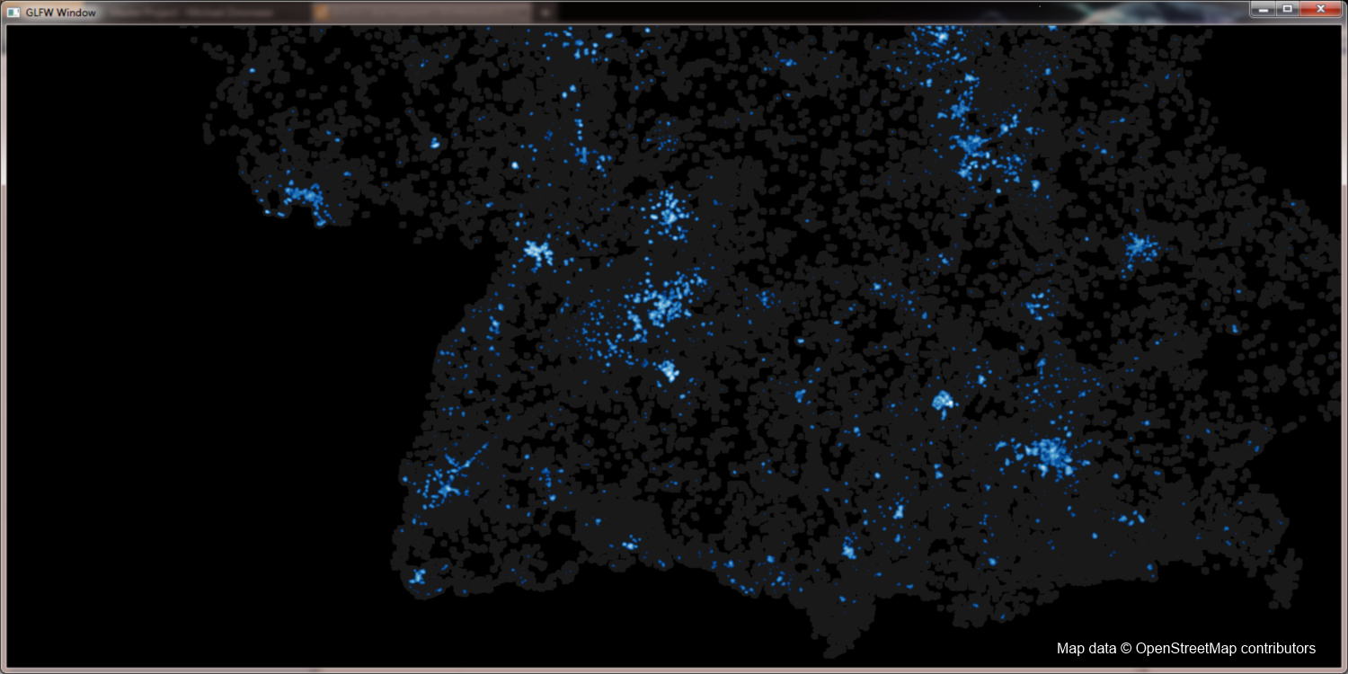
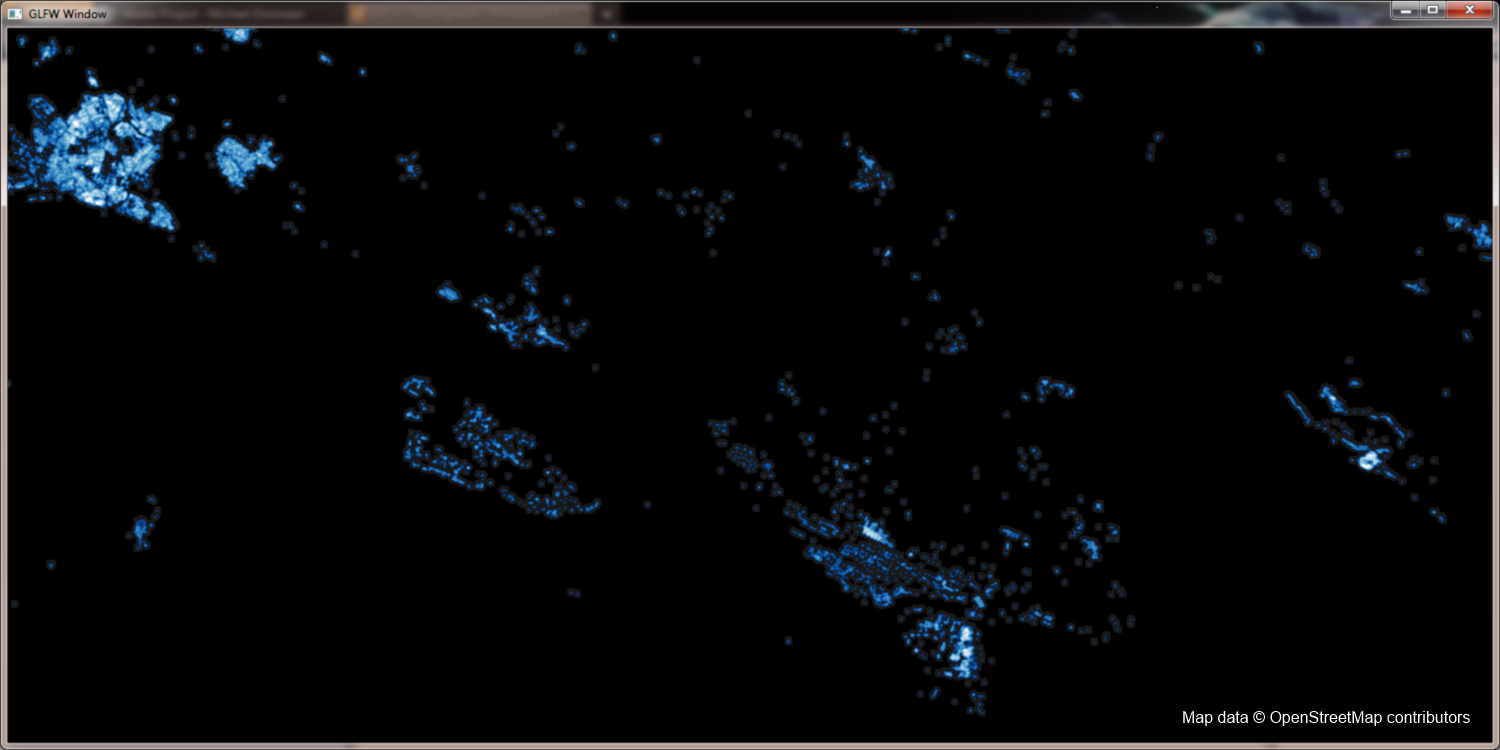
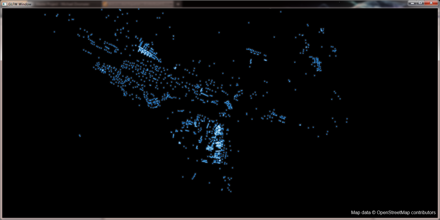
With the help of QuadTrees (see implementation) it is possible to load much larger data sets. One example is the germany data set displayed below. Each point symbolizes one building (source Open Street Maps). With appropriate hardware one can even display whole europe with this method. A data set with more than 37 million single nodes.

Buildings of Germany (Map data © OpenStreetMap contributors):

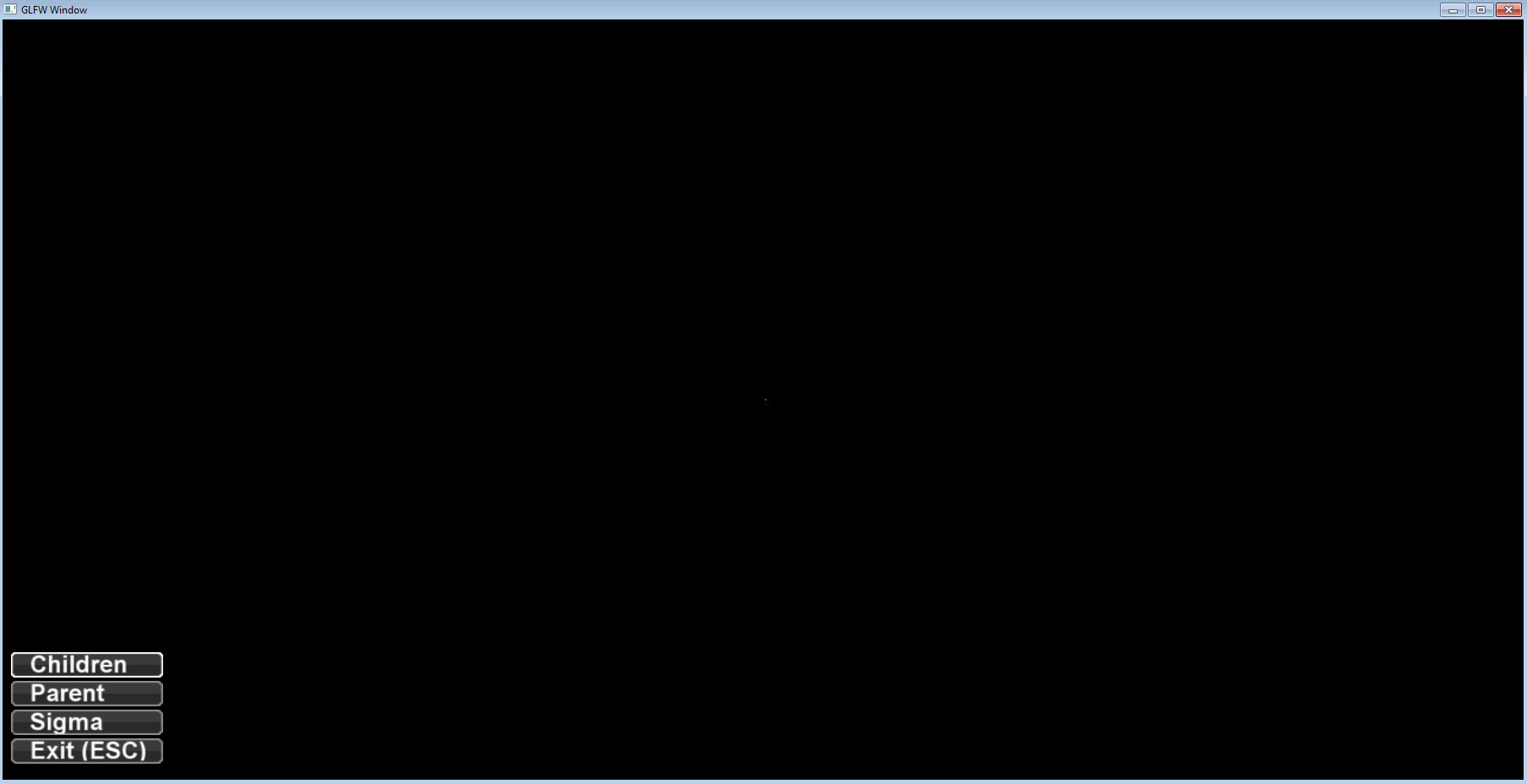
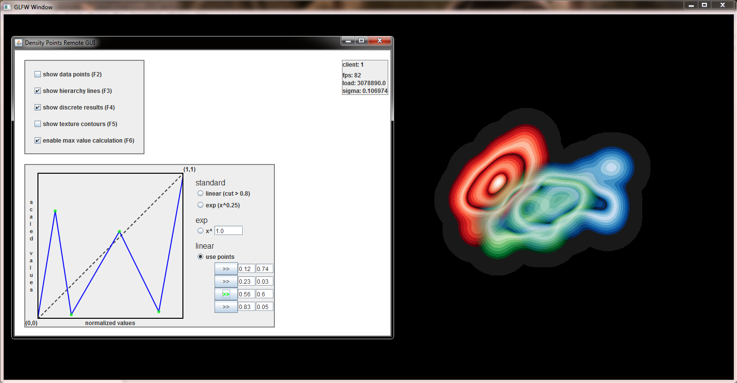
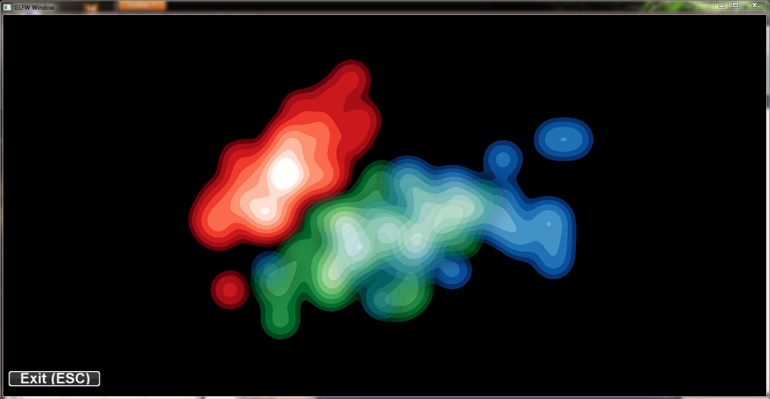
project DensityPoints - Remote GUI & Scaling

Added a graphical interface for the most important key commands and designed a component which gives the user the ability to intuitively change the scaling. Additionally its also possible to produce beautiful meaningless pictures as can be seen below.

Having fun with the Iris/Aids data set:

project NormPoints 2 - Multiple Fields

The Iris data set rendered with three distinct density fields. The clusters differ in their color and shape. Notice the red and blue points in the lower left corner, both disconnected from the green cluster.

Iris data set:

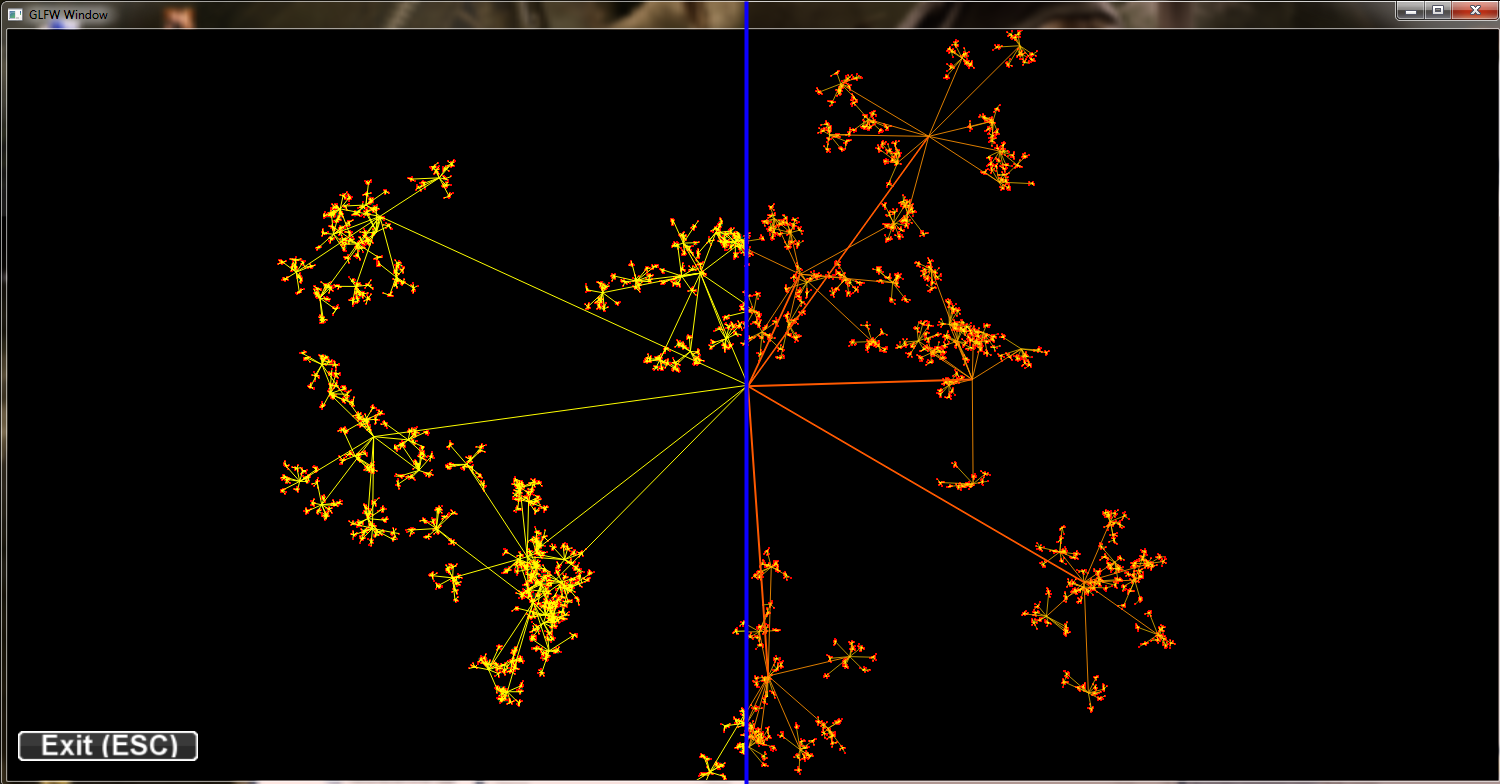
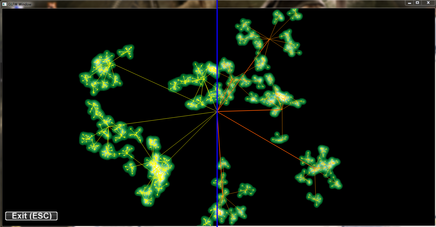
project NormPoints 2 - Improved results

Same hierarchy as below, but with some changes in the rendering process.

• realtime calculated maxValues to normalize the textures
• improved visual perception of tree levels
• floating point texture set for blending

pictures are devided in the middel right side shows the improved rendering:

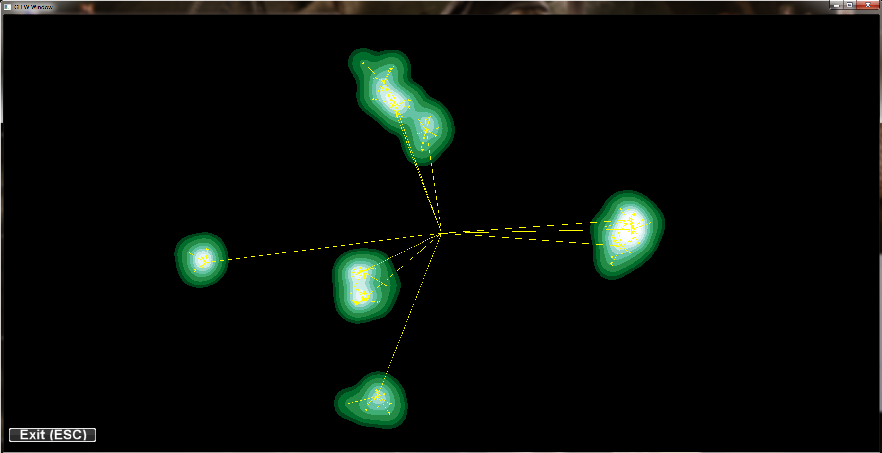
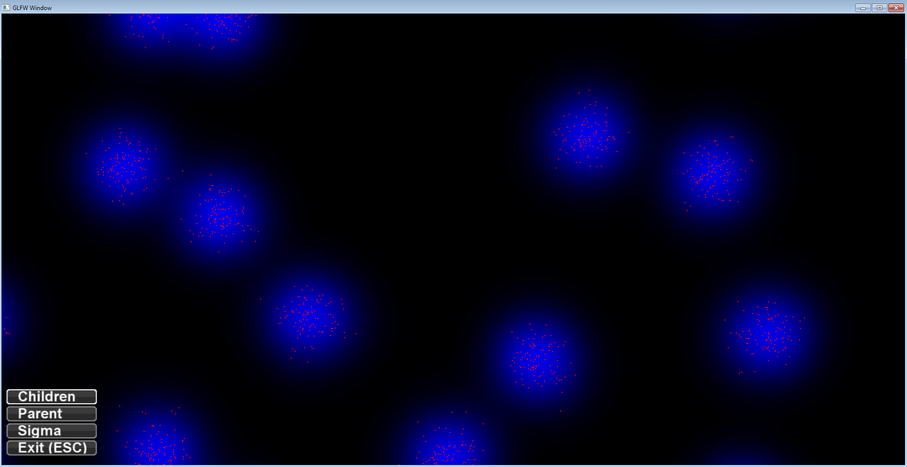
project NormPoints 2 - Hierarchy2

Again a hierarchy picture, this time with 10.000 points on the ground level. The used conversion shader outputs the aggregated blue values. Sigma decreases with a factor of 0.2 and the starting sigma is screenHeight / 3.0.

sigma differs to highlight the clusters:

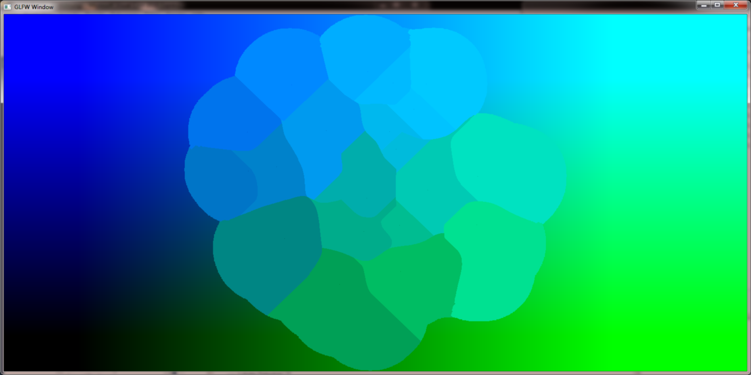
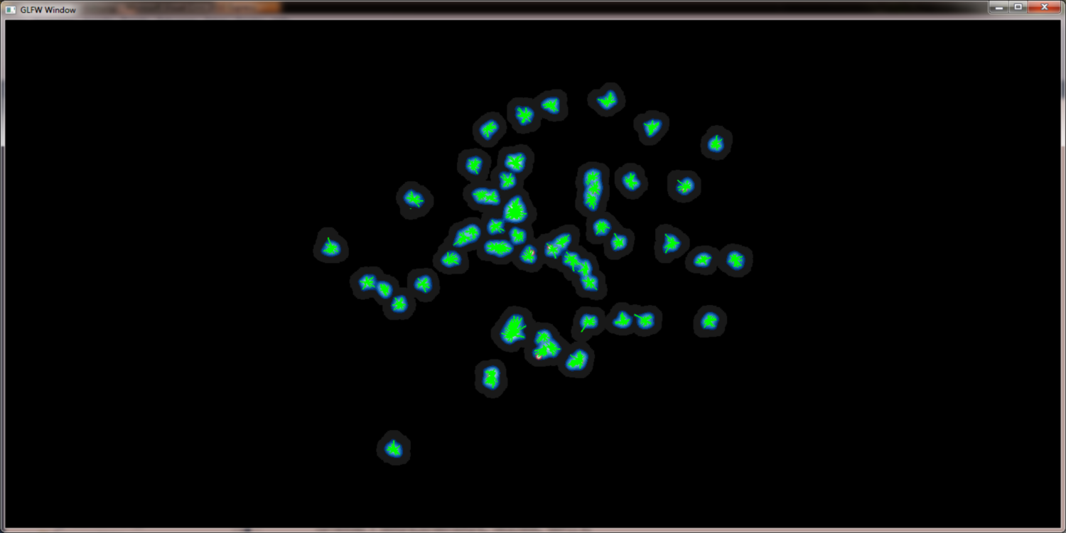
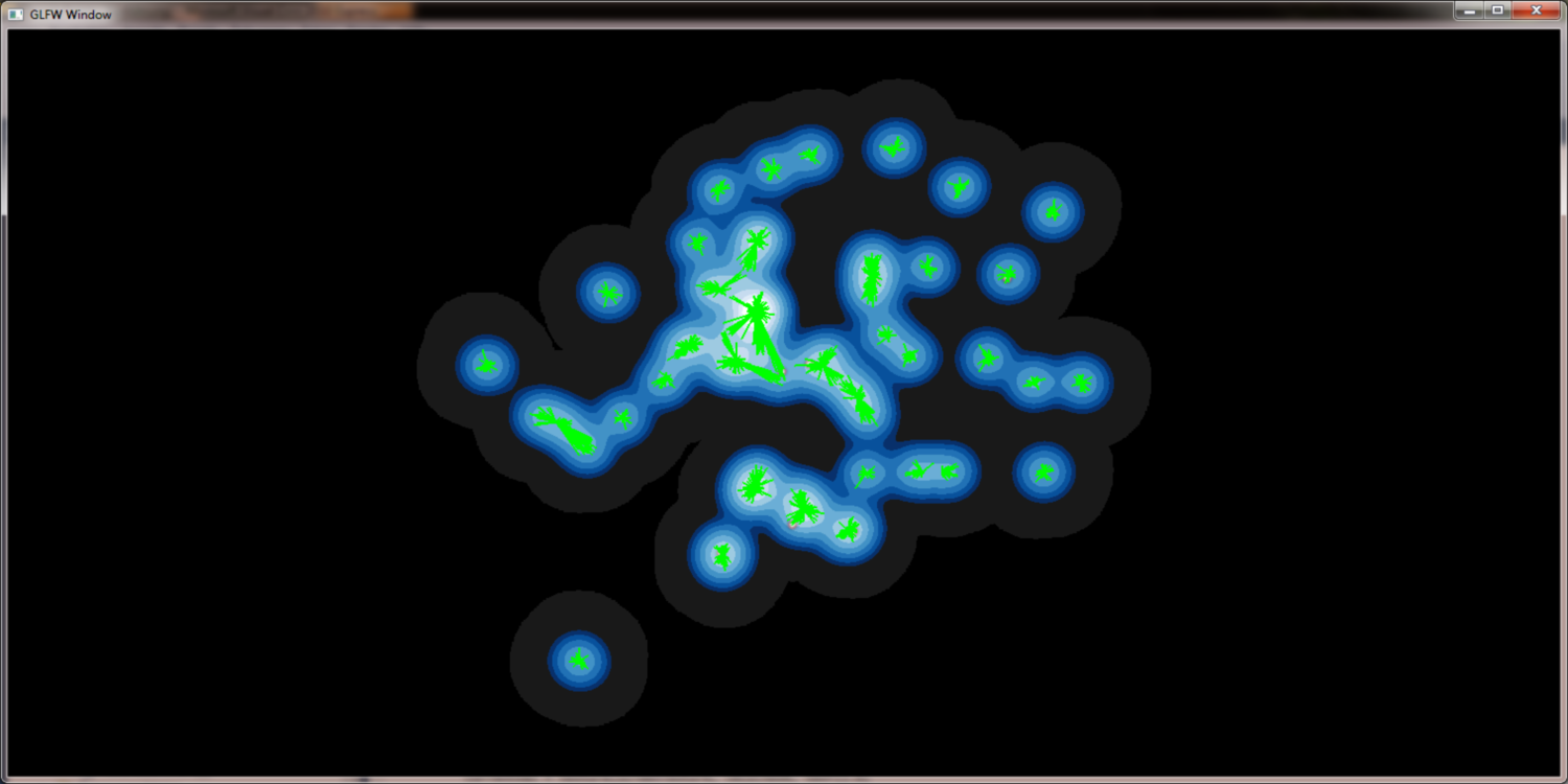
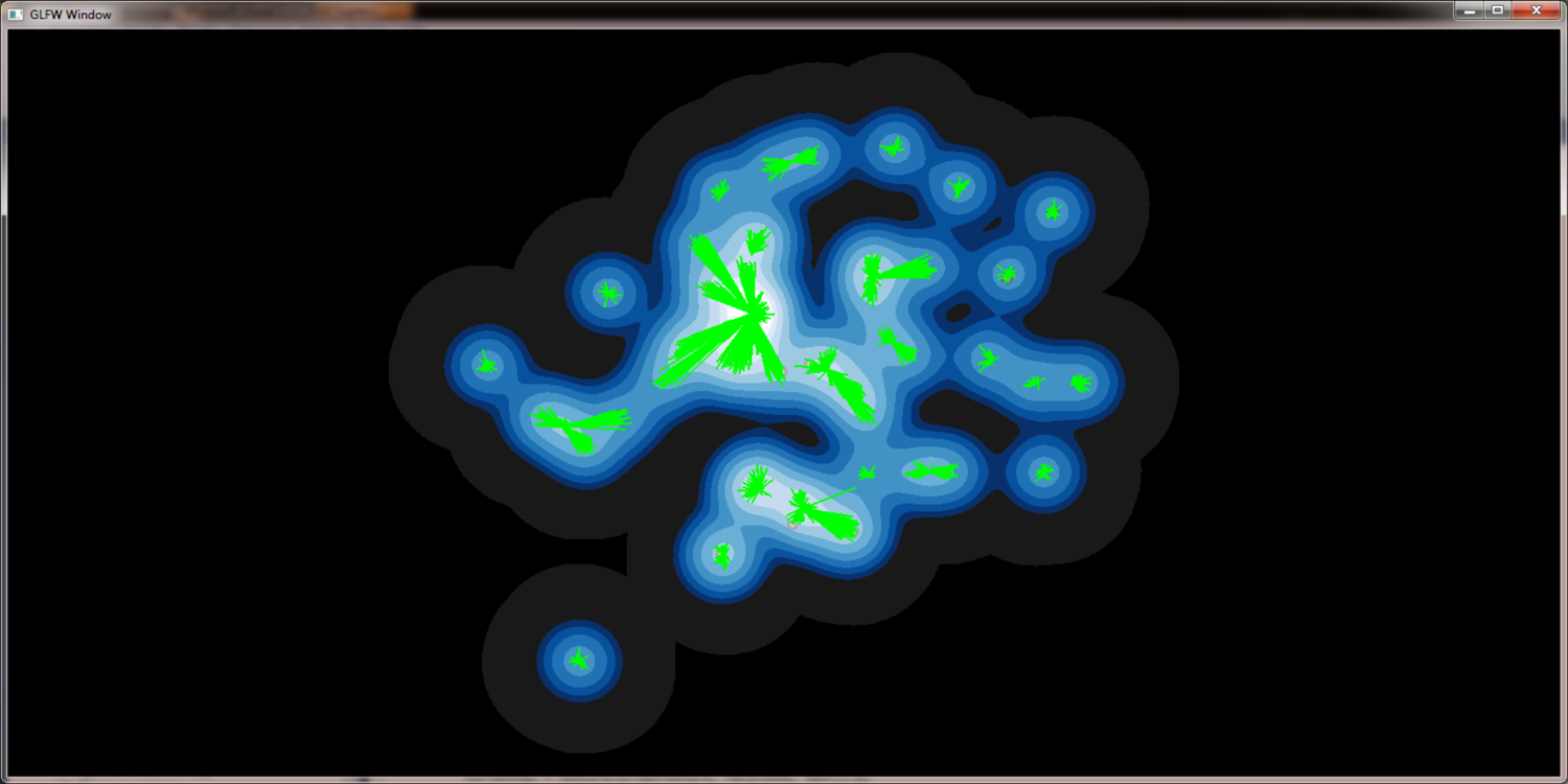
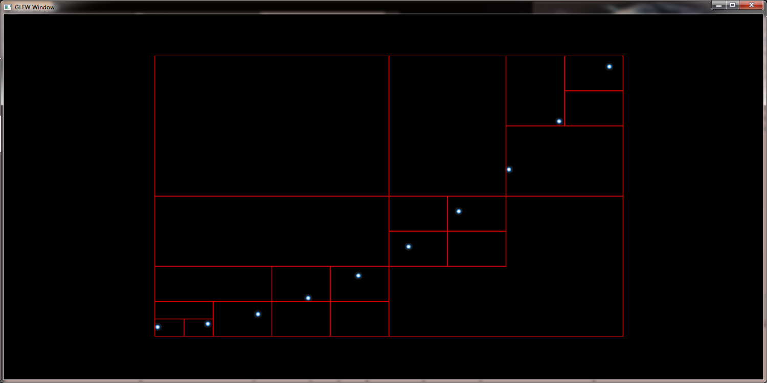
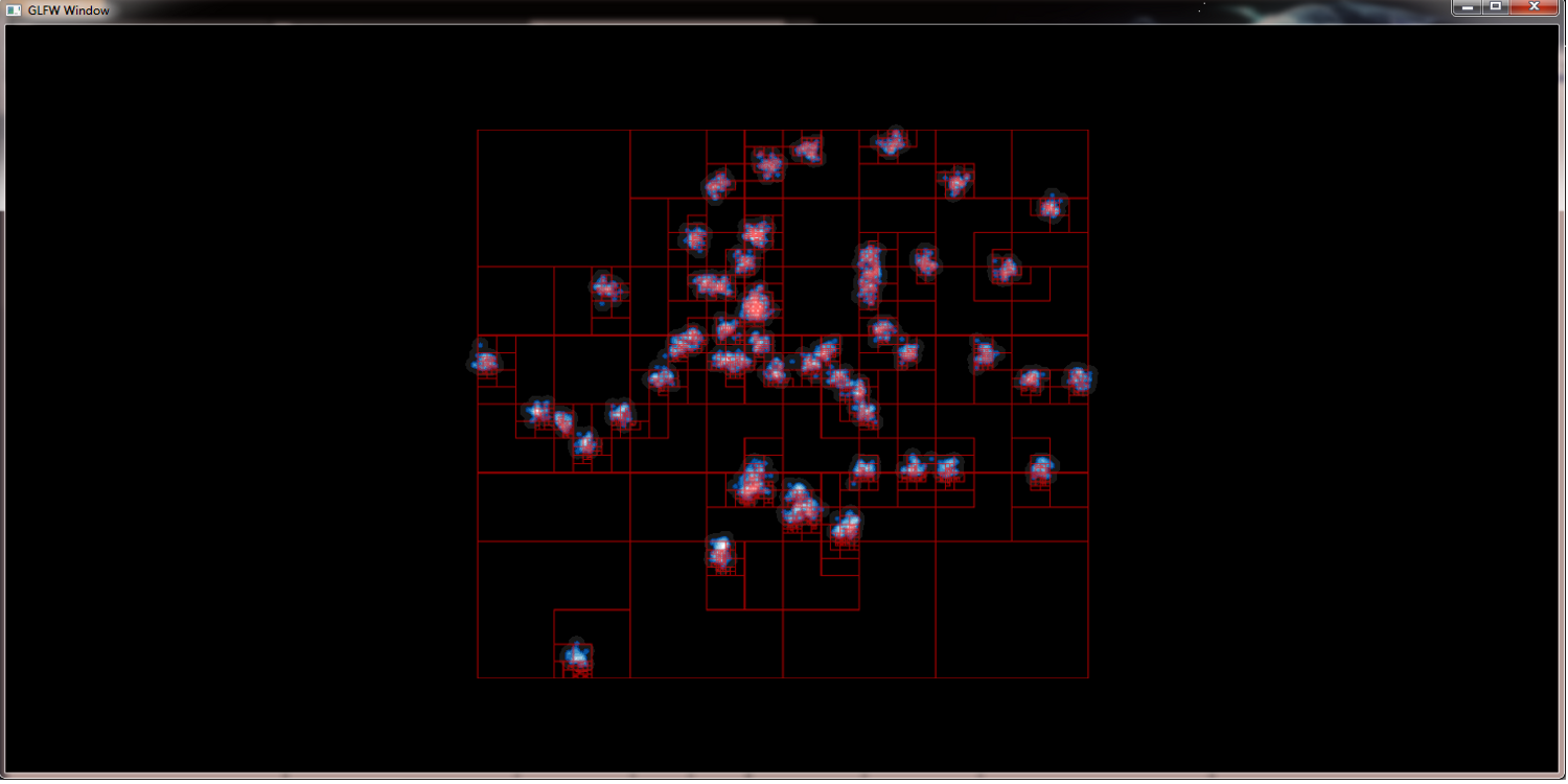
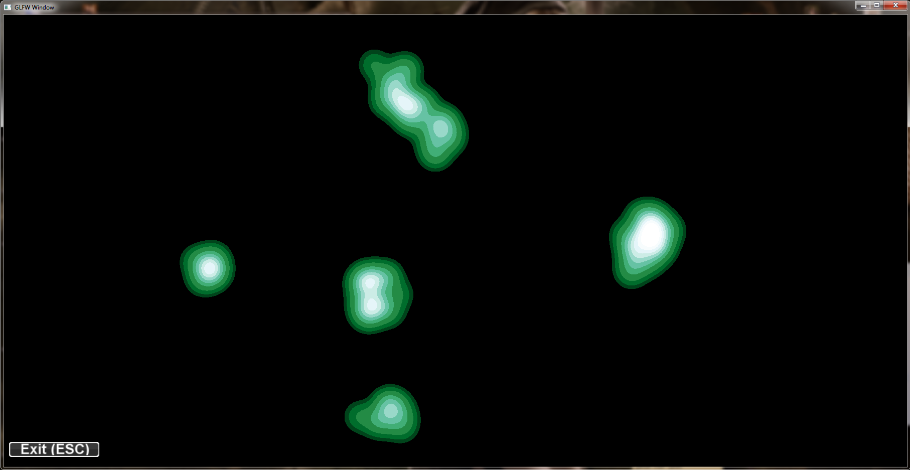
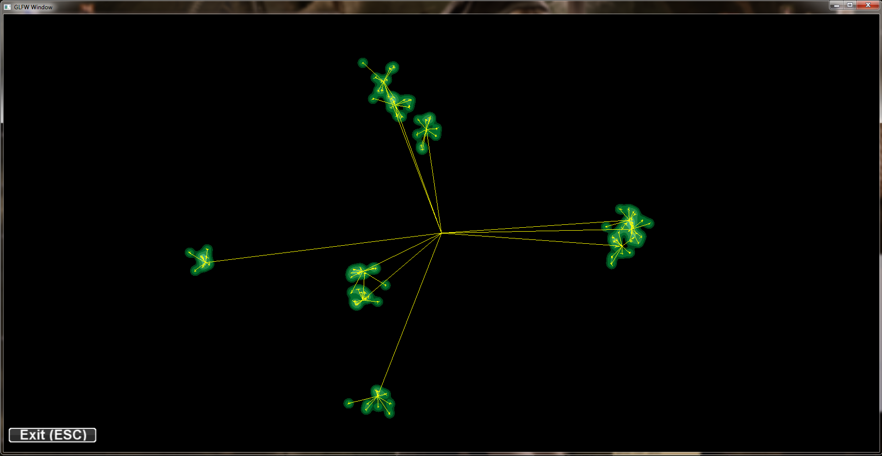
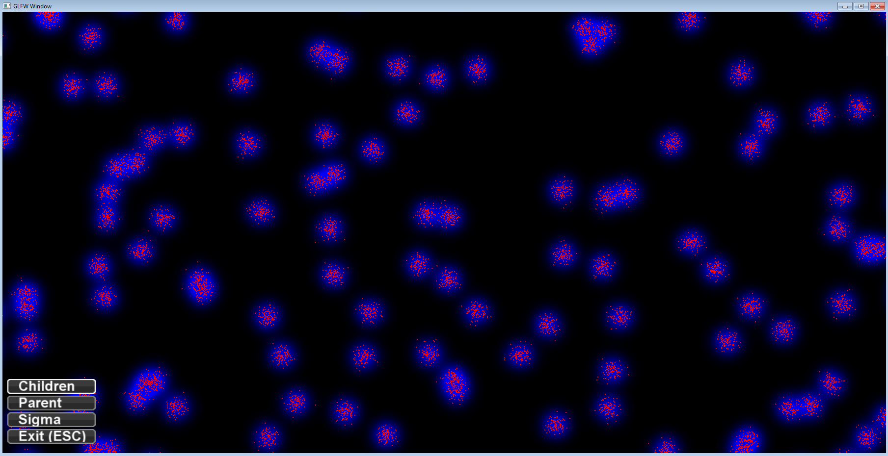
project NormPoints 2 - Hierarchy

Implementation of a hierarchical point distribution; the pictures show three levels each parent having 10 children and sigma starting with a value of screenHeight / 6.0. Sigma decreases by a factor of 0.1 on each level. Only the last level with 1000 points is drawn.

sigma differs to highlight the clusters:

same pictures as above but this time the generating tree is plotted too:

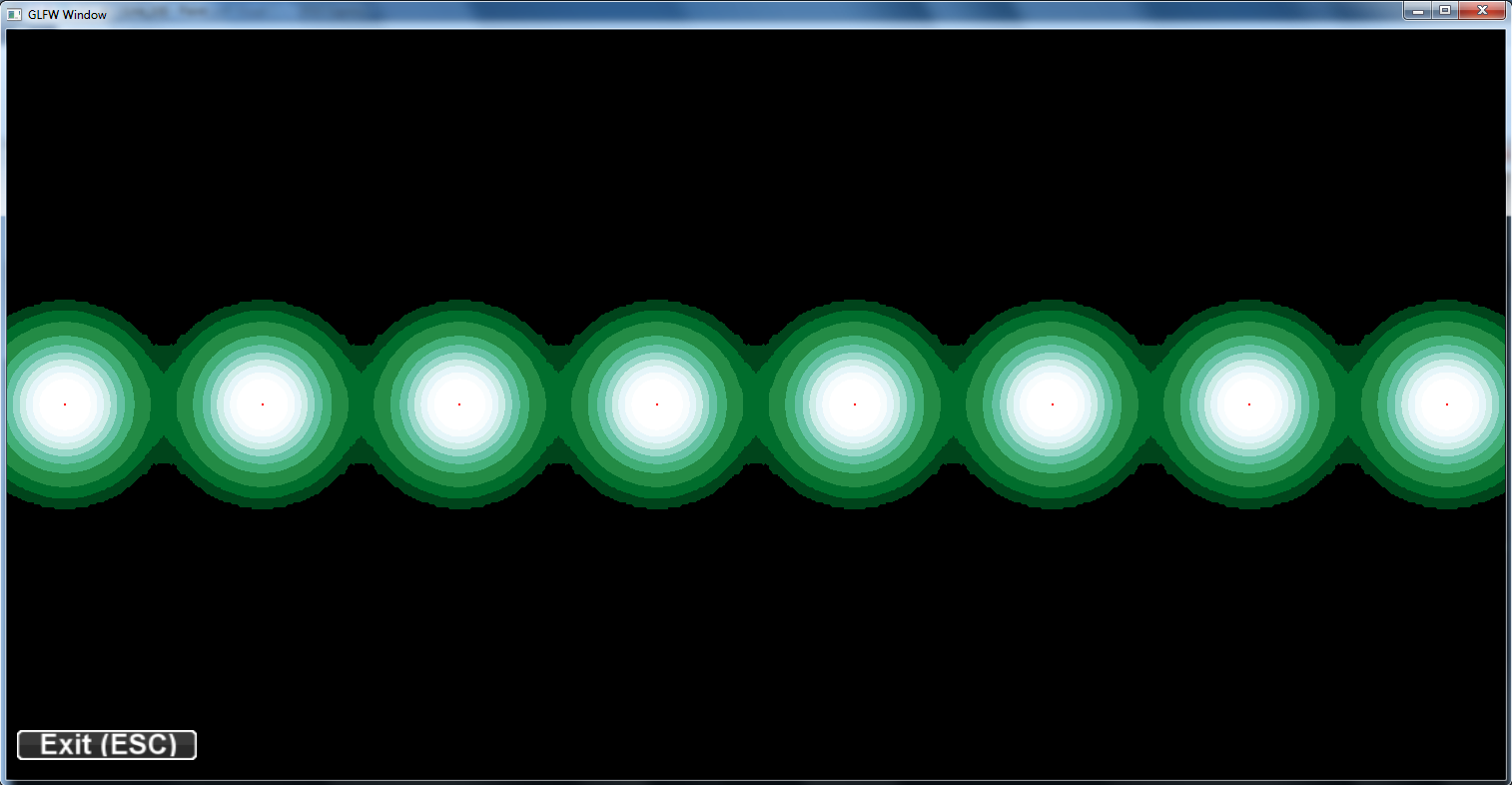
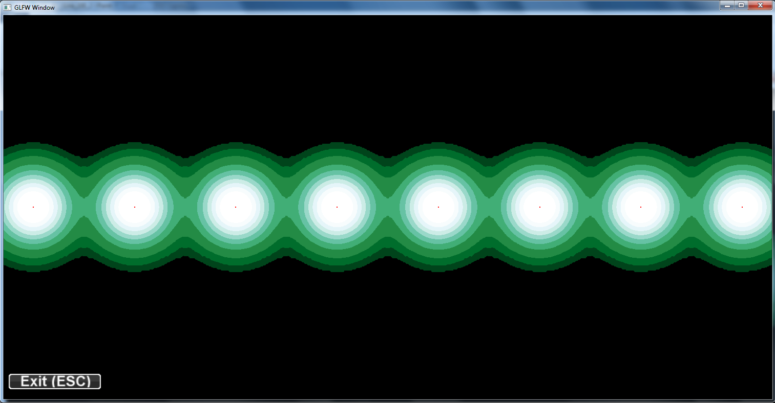
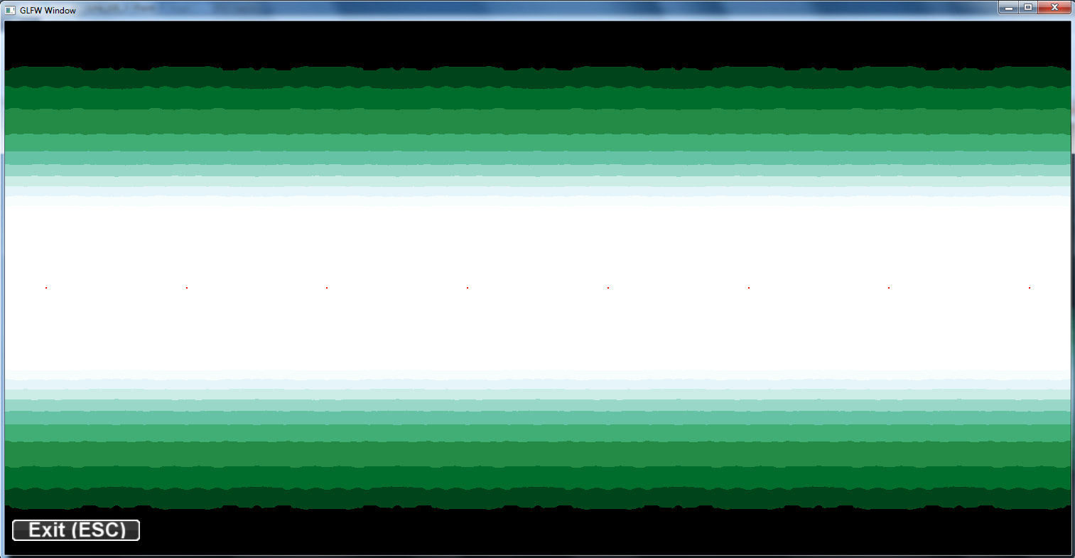
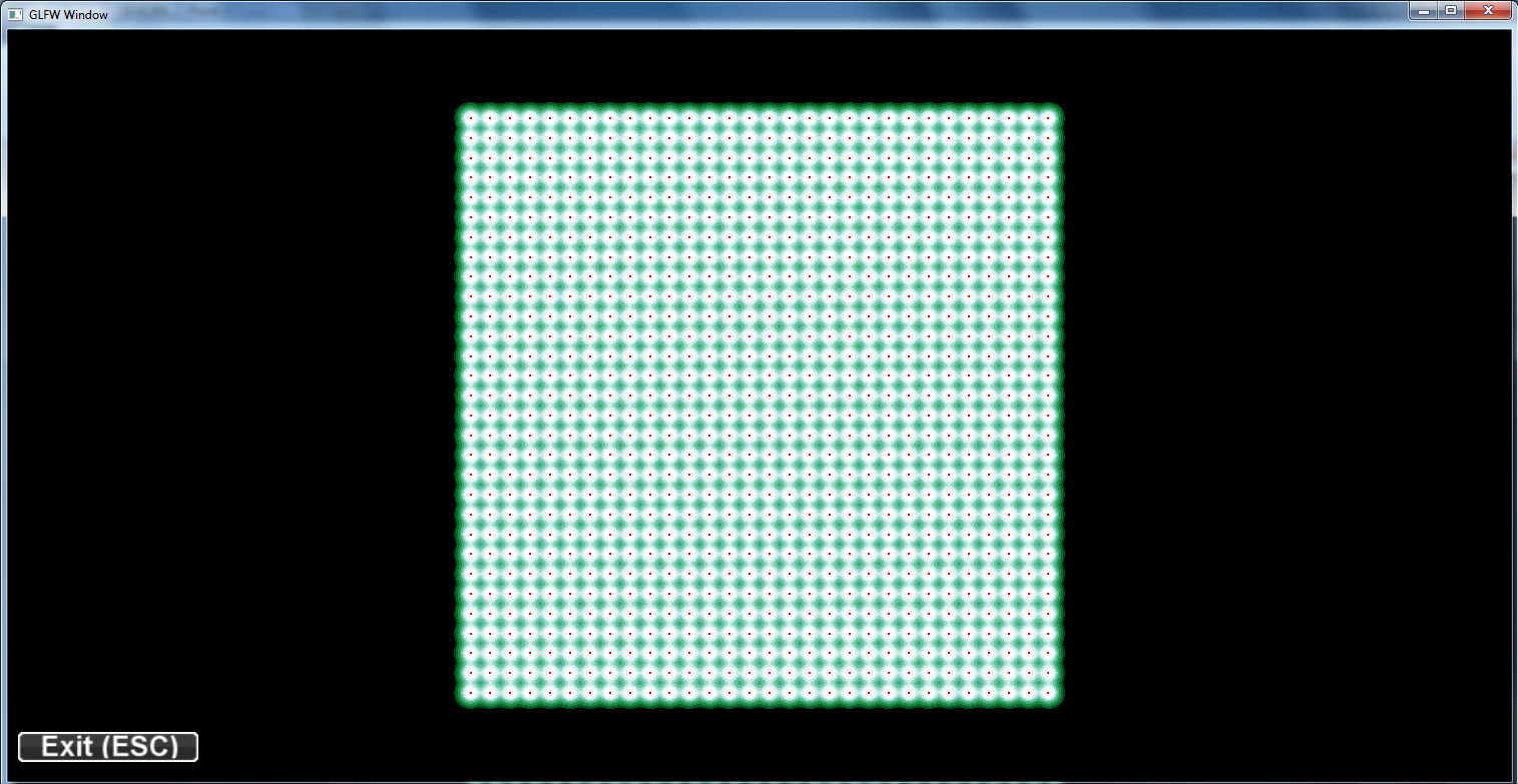
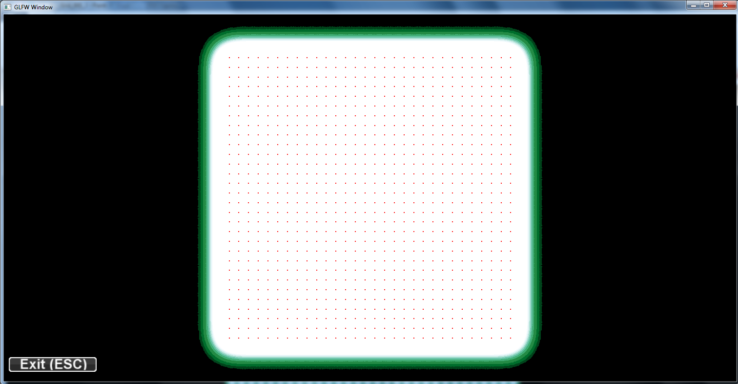
project NormPoints 2 - Grid and Line

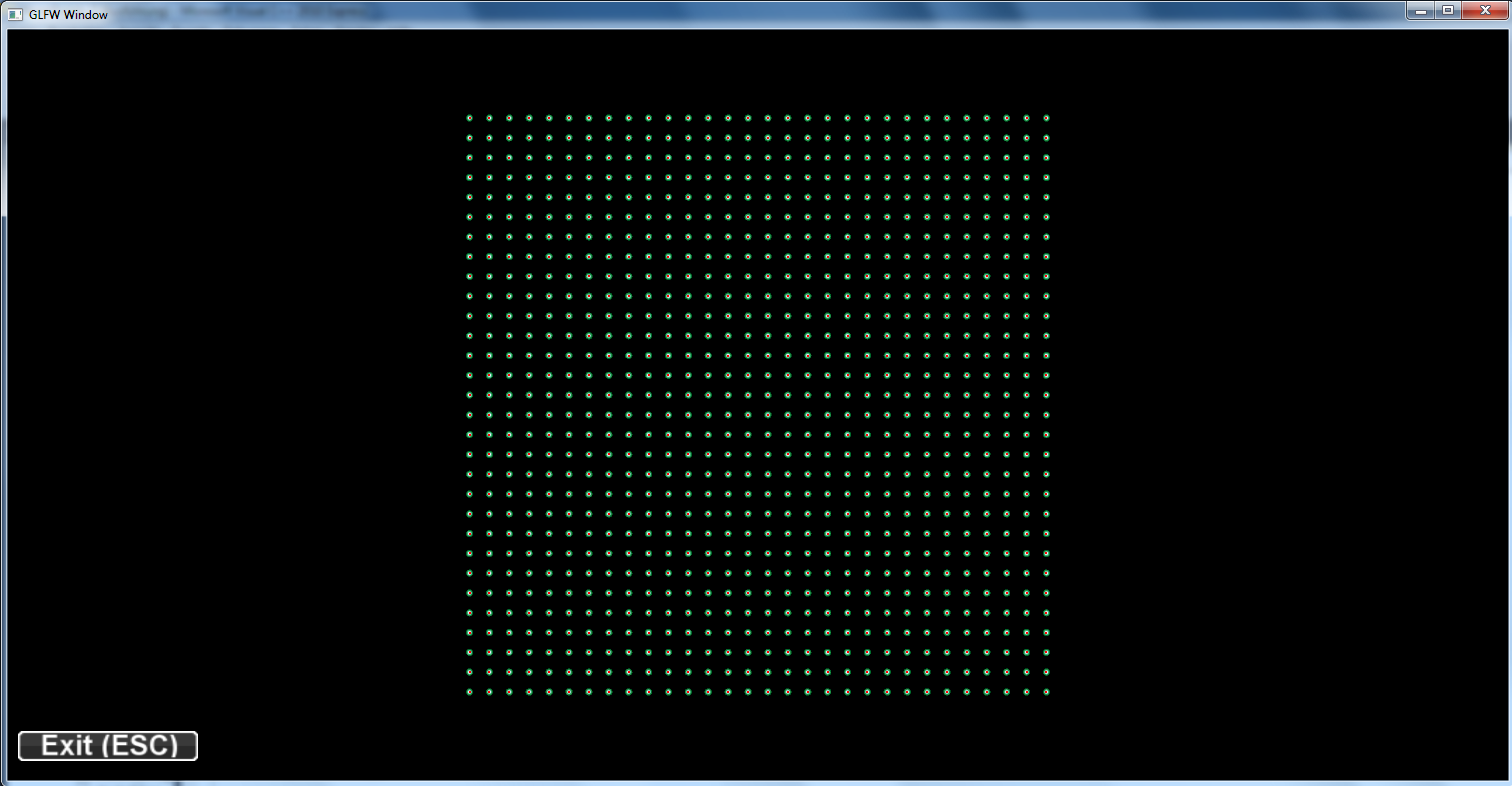
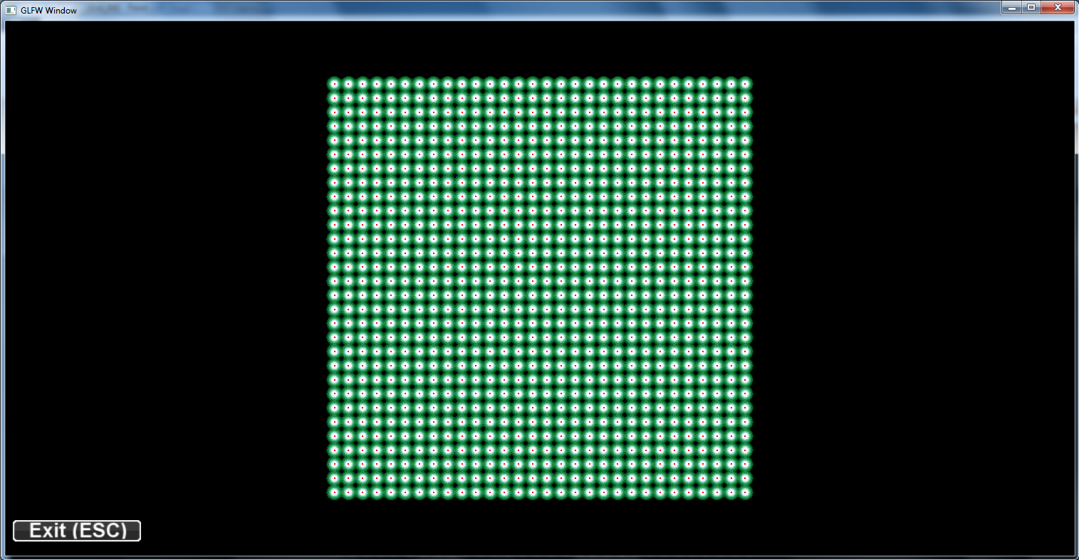
To be able to detect "clusters" we require a variable user specified sigma setting for the gaussian kernels. Sigma starts with a relative small value and can be increased / decreased with the mouse wheel. Examples of the results are provided on data sets of a regular grid (900 points) and a straigth line (100 points).

different sigma levels on a line of points:

different sigma levels on a grid of points:

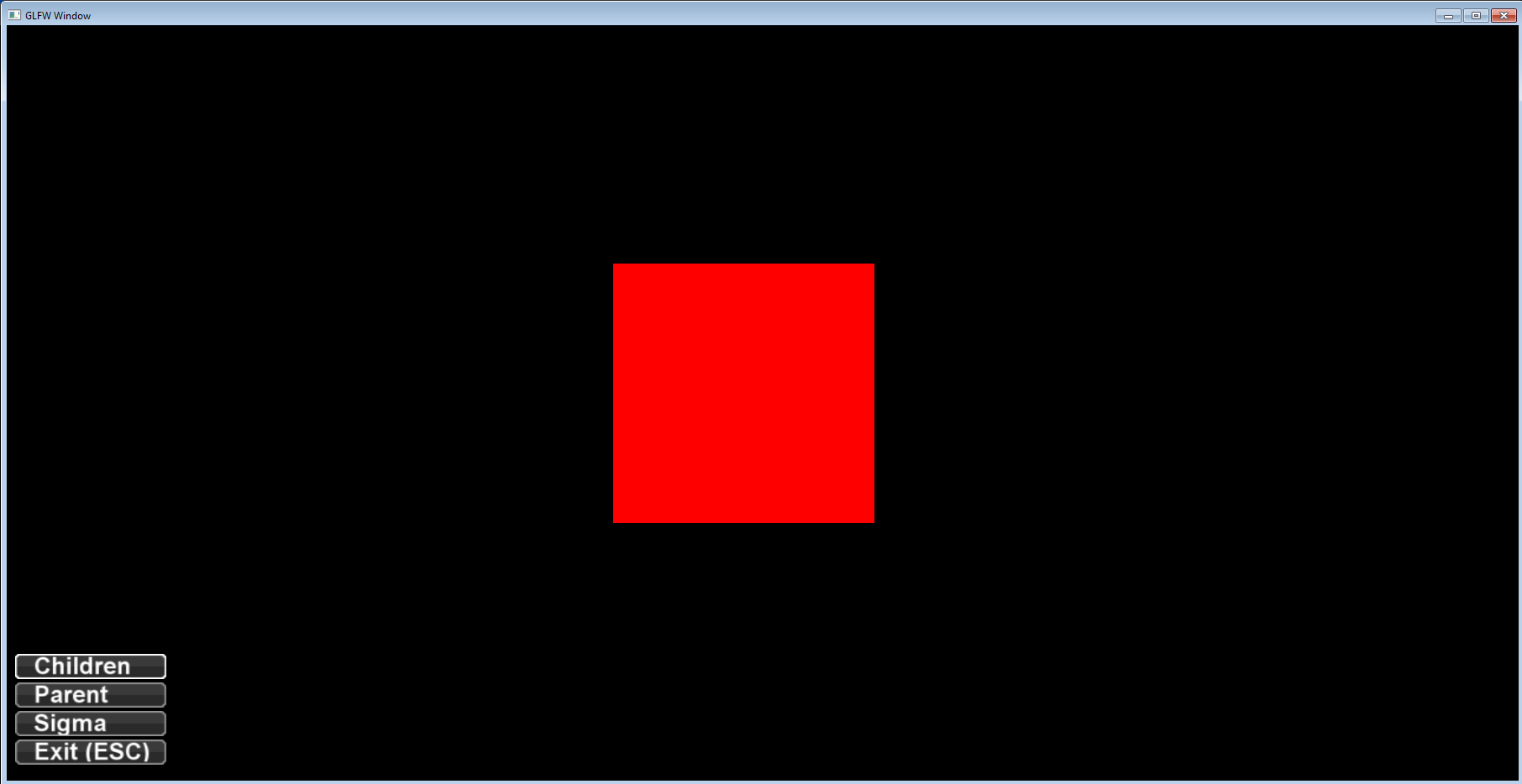
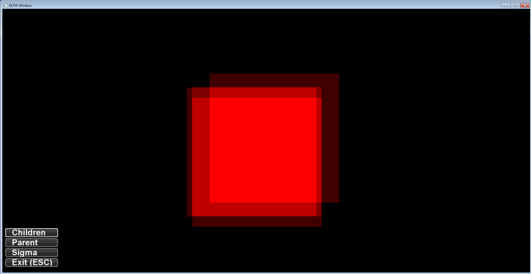
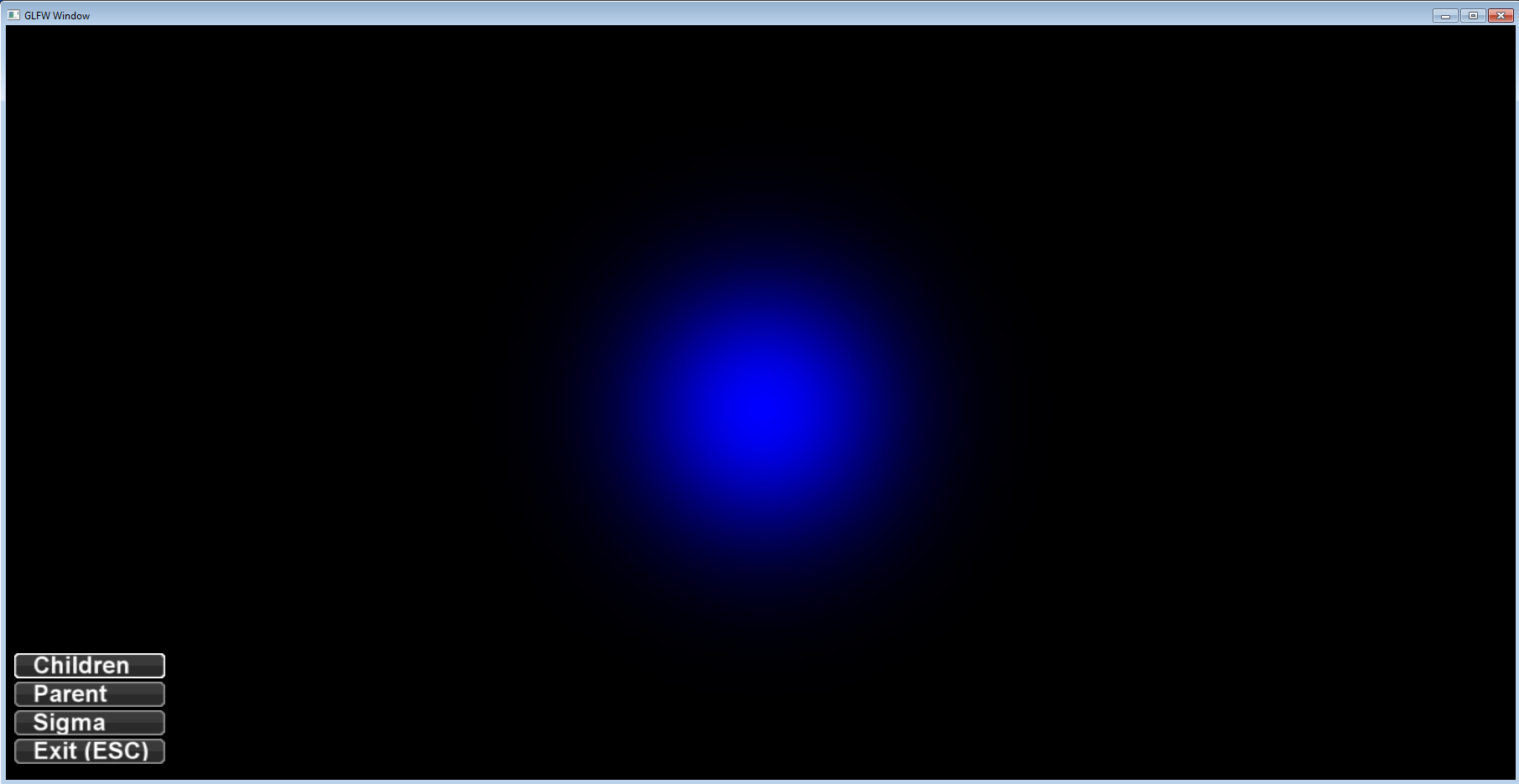
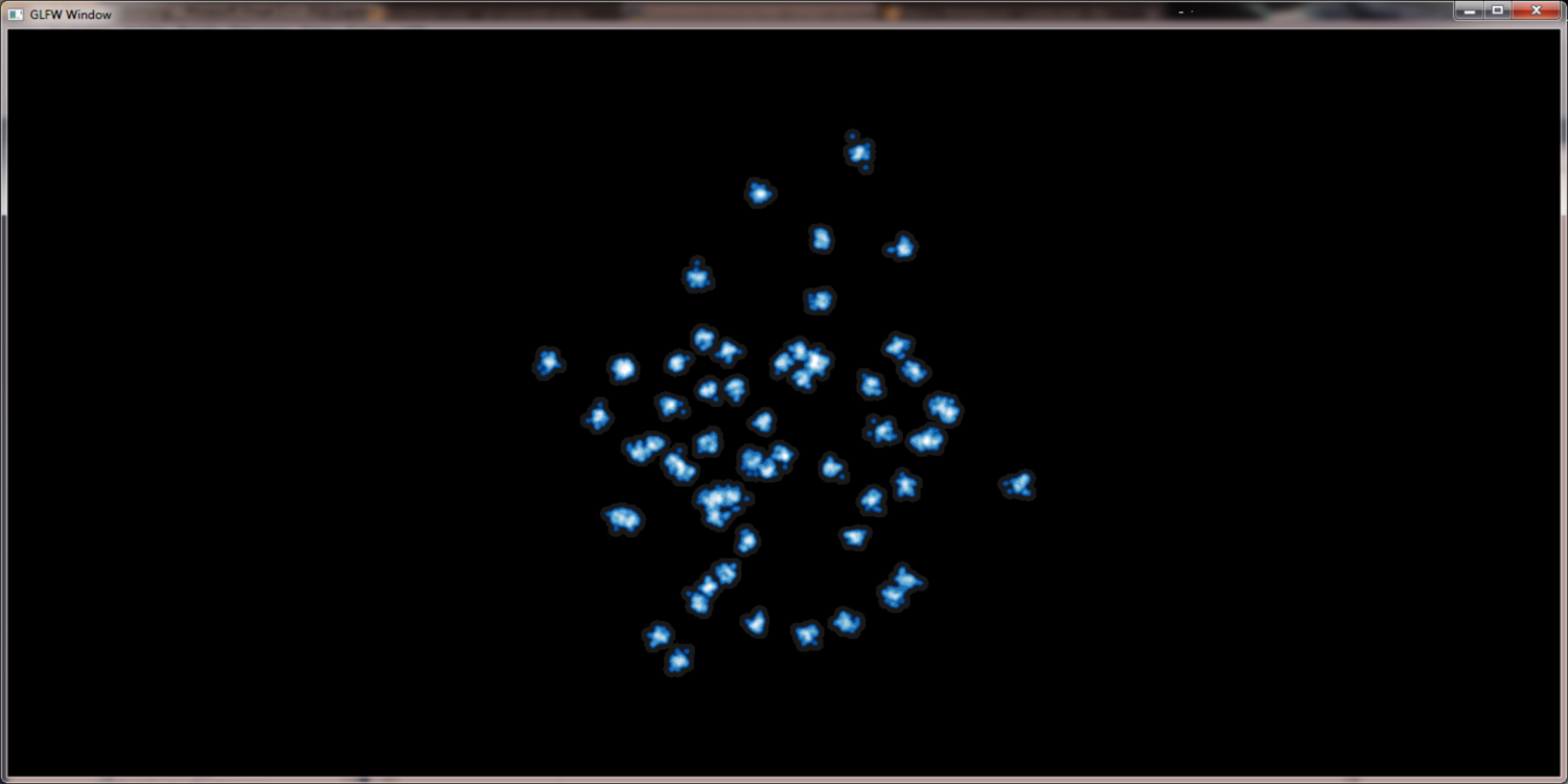
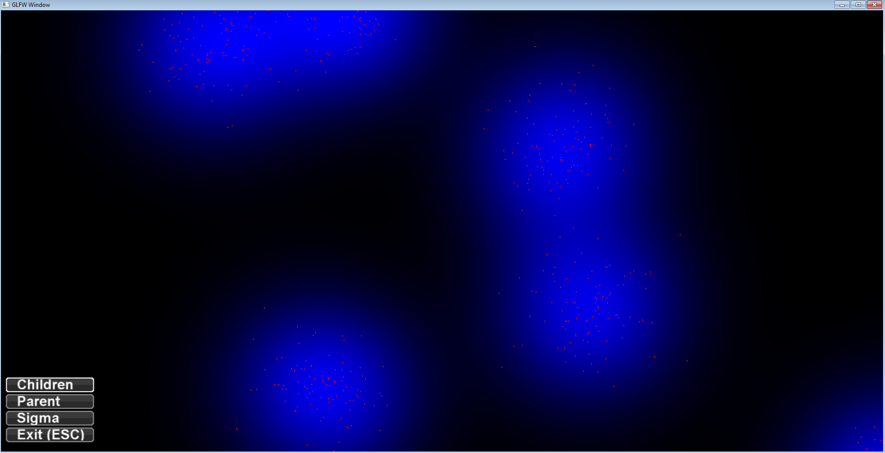
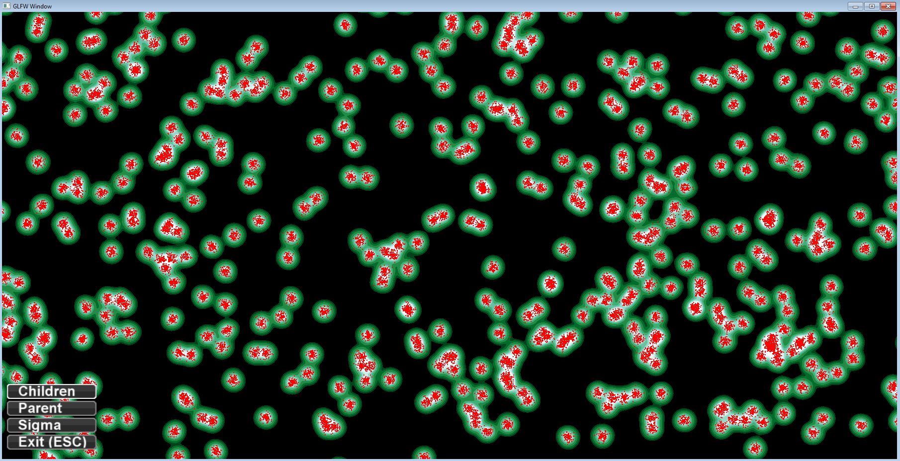
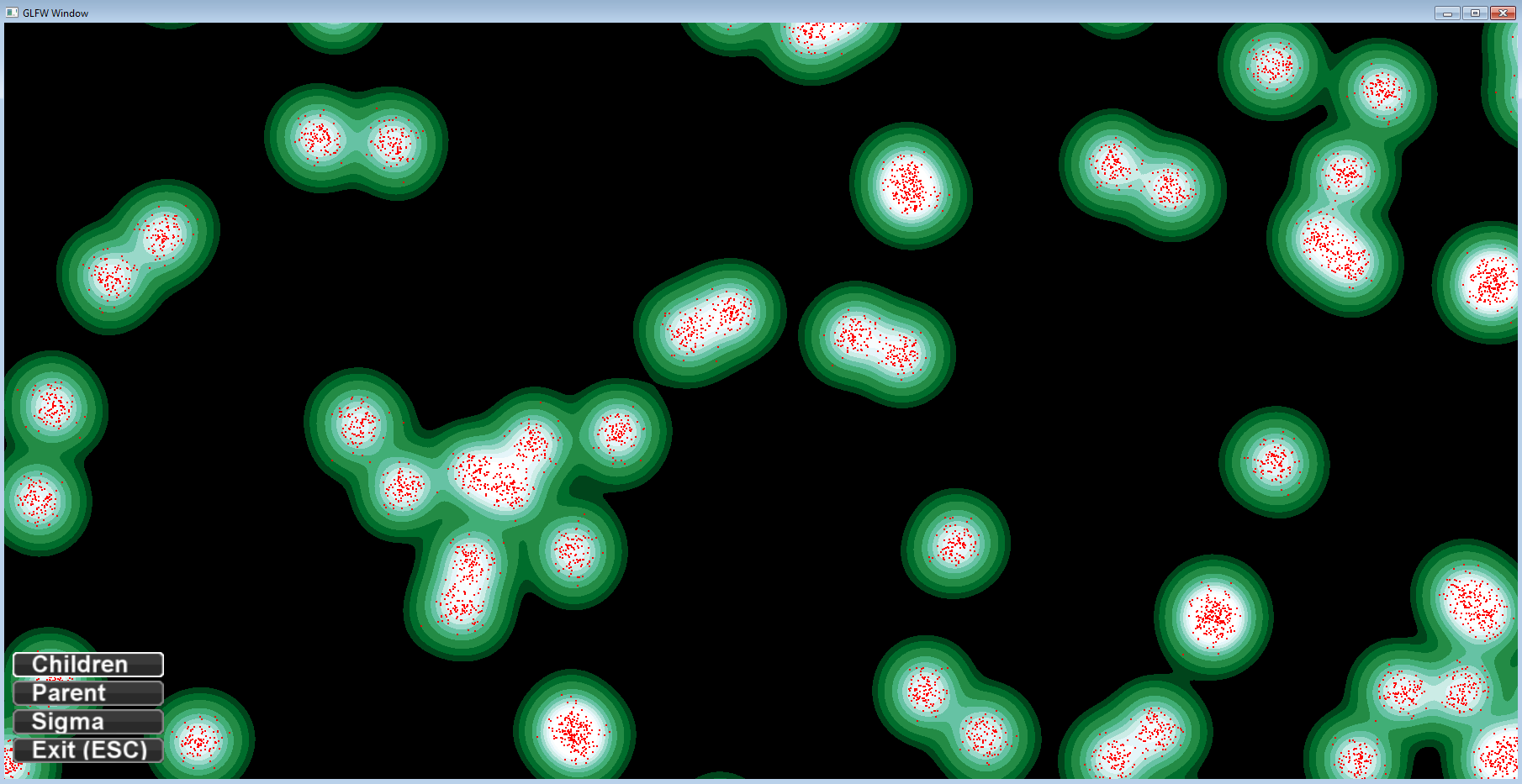
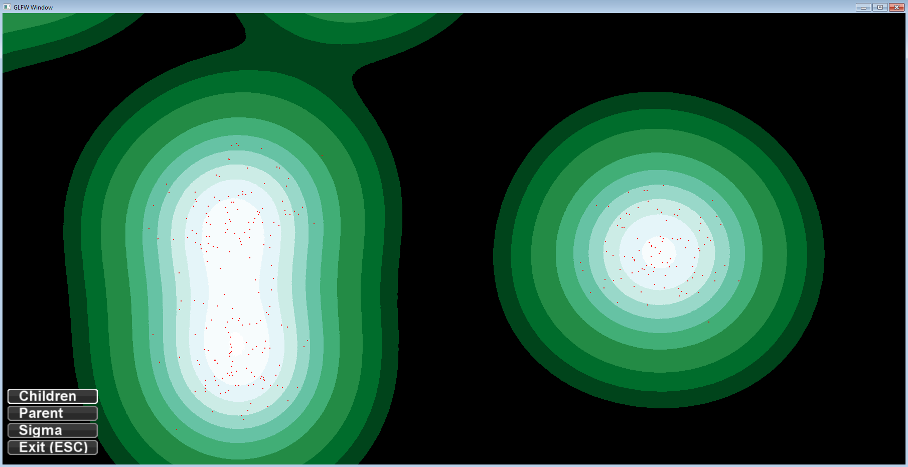
project NormPoints

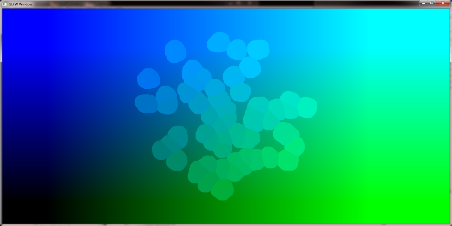
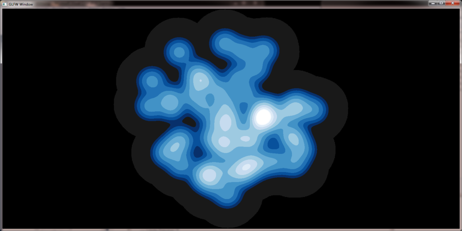
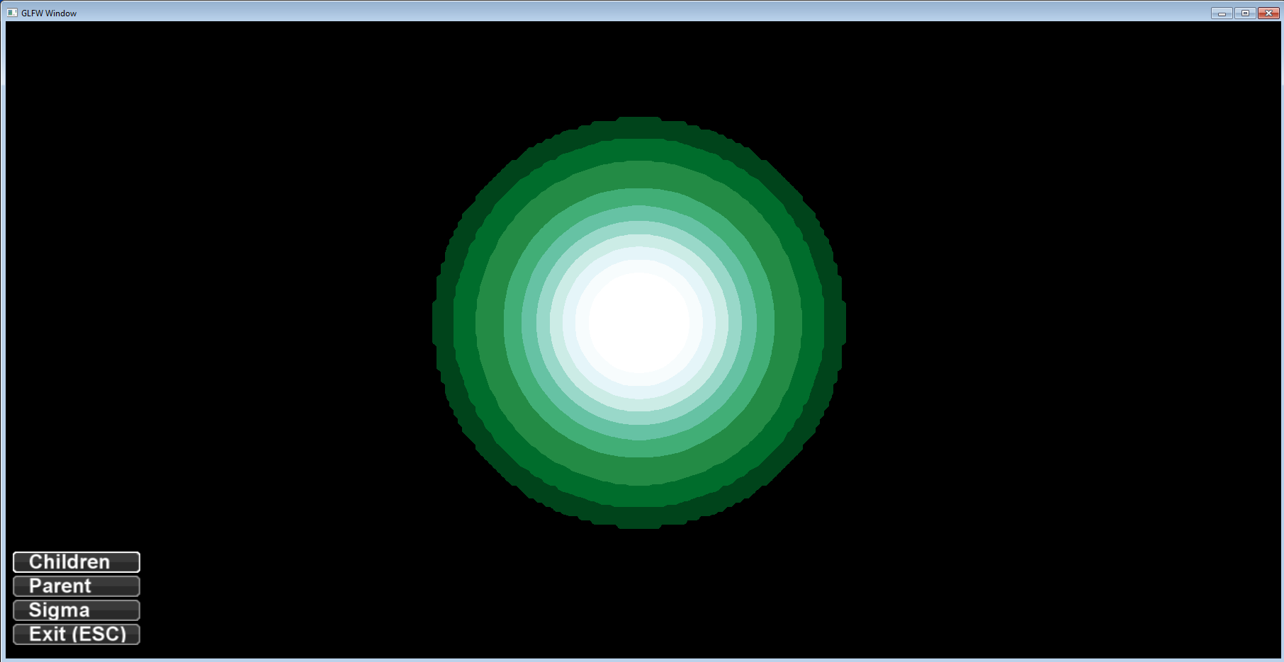
The following pictures show a set of uniformly distributed points having 100 normal distributed child points each. The child points are shown in red and the result of blending togehter their gaussian kernels is shown in blue (direct mapping of values) or green (discretized).

different zoom levels of the gaussian fields arround the child points:

discretized gaussian fields:

Master Project Report: Short description of the techniques that have been used/developed during
the master project in order to prepare the master thesis and the InfoVis 2012 publication.

get it

______________________________________________________

all contents are property of Michael Zinsmaier